This article is probably worth reading twice due to my style of writing (sorry). Read the comments as they have alot of informational text. I tried to make them understandable to a beginner python user/linux hacker.
Before continuing I recommend checking these out – basics on plotting using Python:
http://www.ucs.cam.ac.uk/docs/course-notes/unix-courses/pythontopics/graphs.pdf
http://www.ast.uct.ac.za/~sarblyth/pythonGuide/PythonPlottingBeginnersGuide.pdf
NOTE: all of the above links save the plots to the screen, so you need some sort of Xserver or Desktop system for that. But sometimes your data collector & plotter is nothing more than a server without a monitor. So instead of plotting to a screen we need to plot to a file and then send that file over to a webserver for later viewing.
There are 3 steps in collecting and graphing data. I can generalize them as this:
Step 1. Generate / Collect Data into a file (via bash)
– The general format is that each line has the data from 1 point in time. Or if time is not represented, then each line represents whatever the x axis is (usually with data collection that is date/time)
Step 2. Repeat 1 as many times as needed (via cron)
Step 3. Graph data (can be done after 2 or after 1 or at anytime after *)
a. Read Collected Data (via python)
b. Parse Collected Data into variables (x and y for the graph) (via python)
c. Graph the variables to a plot/graph (via python)
d. Save the plot/graph to a file (via python)
e. Send plots to webserver (optional) (via bash or python)
* Graphing of data just needs to happen as long as there is 2 or more data points.
In this example we will go through each step using an example. Then at the end there will be extra examples of step 3 of graphing different types of collected data – which is the more complex step.
*** FIRST EXAMPLE ***
0. Get all of the tools needed for the job
Step 0 was not included in the generalization at the top as this is only required once. Here we will download the needed programs to get this done.
COMMANDS:
# update the repos (hopefully you have the write lines in /etc/apt/sources.list - if not then none of the following will download)
apt-get update
# install the packages one by one (I find that its better than stringing them all together - when you string them I find that apt can skip some)
apt-get install nano
apt-get install vim
apt-get install python
apt-get install python-matplotlib
apt-get install python-matplotlib-data
For later use in the python script (which will do the plotting), we need to get the name of default font – or else everytime the python script is ran a warning is shown that some font wasnt found so the system is using the some default go-to font. This warning can be avoided by setting the general font of the plotter to the default go-to font of the system.
1. Generate / Collect Data:
Lets collect some system information and plot it. For the sake of simplicity we can use a bash script to collect this data.
0. date/time (this will be our x axis)
– The best date and time to collect is unix epoch time, however we can also collect regular dates for human readable understanding
– With linux this can be done using “date” for human readable time. And “date +%s” for parse able date (its just the number of seconds that has passed since the milestone marker of Jan 1st 1970)
1. uptime
– The command that we can use for this is “uptime” or get the data from /proc/uptime using “cat /proc/uptime”.
2. free ram
– We can get this data with “free -tm”
3. load average
– We can get this data with “uptime” or with “top -cbn1” (which is a good command to commit to memory as it basically runs “top” but only once, hence the -n1, and with no color/special character highlighting, hence the -b, and it also shows the full command names & their arguments, hence the -c)
4. free space of a volume
– We can get this with “df -P -k”. We use -P because df sometimes splits single entries, that are too long, into 2 lines, with -P it will not do that, we use -k so that the space is always in kilobytes, or else we have -h output which can shift units to make it more human readable. We want to maintain the same units on each data point inquiry.
All of these variables will be saved into one line and appended into our data file (we will call the DATAFILE /root/script/data-ex1.txt). Each time this script is ran that data file will be 1 line longer. Each line will be something like this:
date|date|uptime|freeram|loadaverage|freespace of a volume
That would be a simple data entry line. So in the end, after a year of running, it would be like 1000s of lines of this:
Mon Apr 13 23:16:12 PDT 2015|1428992172|8862.03|2215|1.75|1803072512
We could, of course, make the data be easier to read in the DATA FILE by making it look like this.
* date: Mon Apr 13 23:19:56 PDT 2015|1428992396s|uptime: 9086.24|freeram: 2213mib|1.05 loadavg|1803072508 KiB freespace on /data
However if we make the DATA FILE easier to read, it will only make parsing the data in the python file harder (but still doeable)
This example will focus on the simple entry style: March 17, 2015|17000000|123123|456|1.5|5000000
The other Examples below will show how to parse data in more complicated DATA FILES.
So for the sake of keeping the first example more simple the DATAFILE will be single character delimited with the pipe symbol “|”. Keep in mind: most data files (especially csv files) the most common delimiter to be used is the comma “,” or the space ” “.
COMMANDS:
# make the folder for the scripts
mkdir -p /root/script
# write the data collection script - opening the nano or vi editor with the first argument being a non-existant file will imply that your creating a new file
nano /root/script/data-ex1.sh
# now write the script below into that file
chmod +x /root/script/data-ex1.sh<span style="font-family: Lato, sans-serif; font-size: 16px; line-height: 1.5; background-color: #ffffff;"> </span>
SCRIPT /root/script/data-ex1.sh:
stuff#!/bin/bash
# filename: /root/script/data-ex1.sh
# this script collects data
DATAFILE="/root/script/data-ex1.txt"
( # I make a subshell with the () so that the variable names I use dont interfere with any system variables that might be in place
DATES=`date +%s` # date in epoch seconds
DATEH=`date --date=@${DATES}` # this is the same as `date` - however I used this more complicated method which matches the human readable date output to whatever the date is in variable DATES. that way if there is system hang between DATES and DATEH, the dates would still correspond.
# DATEH=`date`
# next we use a bunch of greps/awks (and can use seds) to extract the data for the other variables. For online stuff we can use curl and wget (you can even use curl and wget to get data out of websites where you have to login - tip/sidenote, with curl you would need to use -b and -c for keeping track of the login and logout with the cookies)
UPTIME=`cat /proc/uptime | awk '{print $1}'` # seconds
FREERAM=`free -tm | awk '/Total:/{print $4}'` # mib
LOADAVG=`cat /proc/loadavg | awk '{print $1}'` # unitless
FREESPACE=`df -P -k /data | tail -n1 | awk '{print $4}'` # kib
# we only want this to append 1 line to the data file
echo "${DATEH}|${DATES}|${UPTIME}|${FREERAM}|${LOADAVG}|${FREESPACE}"
## if we wanted cleaner data, uncomment below (python parsing script will need to be updated for plotting to work)
## echo "* date: ${DATEH}|${DATES}s|uptime: ${UPTIME}|freeram: ${FREERAM}mib|${LOADAVG} loadavg|${FREESPACE} KiB freespace on /data"
# after we get the one line of output, then we use the command "tee -a" so that the output can be on screen and also appended to the file. Or else if we used >> then we wouldnt see the output on the screen and we would need to "tail" the DATAFILE or "cat" it to confirm
) | tee -a "${DATAFILE}"
2. Repeating 1:
2. For step 2 we have to repeat step 1 so that we get more than set of data – DATAFILE will grow one line at a time each time step 1 is repeated. So that we can see a trend in time. For step 2 we will ask script 1 to repeat. We can use “cron” which is a linux scheduler, to repeat our data collection script. We will ask “cron” to repeat our script once every 10 minutes.
*/10 * * * * /root/script/data-ex1.sh
The next step will be step 3 which is plotting the data. We will make a script called /root/scripts/plot-ex1.sh for that. And we can run it after /root/script/graph-ex1.sh in our “cron” script using this syntax:
*/10 * * * * /root/script/data-ex1.sh && /root/script/plot-ex1.sh
Or we can simply put the following line “/root/script/plot-ex1.sh” at the end of “/root/script/data-ex1.sh” that way we know once data-ex1.sh finished then it starts plotting data.
In our case /root/script/data-ex1.sh will run /root/script/plot-ex1.sh at the end, because /root/script/data-ex1.sh will be a quick to run script (sometimes collecting data takes alot of time, so thats a good time to consider seperating the data collection script from the plotting script)
SIDENOTE: the plotting bash script doesnt do any plotting, the python script will do that
COMMANDS:
# edit the crontab to set the "cron" job
crontab -e
# append below SCRIPT line into the very bottom of the crontab
SCRIPT crontab:
*/10 * * * * /root/script/data-ex1.sh
3. Plotting / Graphing (the python script is here)
Our script “/root/script/plot-ex1.sh” will run the python program “/root/script/plot-ex1.py” which will actually generate the plots/graph (it will first parse the DATAFILE “/root/script/data-ex1.txt”), after that it will send all of the data to a webserver using scp or ssh sending commands (“cat localfile.png | ssh server ‘cat – > remotefile.png'”). From there a user can view the graphs on the webserver. Every 10 minutes the cycle will begin again where “/root/script/data-ex1.sh” is ran to collect data and then the data is plotted via “/root/script/plot-ex1.py” and sent on to a webserver.
SIDENOTE: Here we have 2 bash scripts. One for collecting data and one for plotting the data. In reality those 2 can be put together into 1 – where we first collect the data and then plot the data. However I like to have the plotting script seperate, because sometimes collecting the data takes time and needs to be done religiously on a cycle, where as plotting the data should be done freely and whenever you want (i.e. like after changing the look & feel / layout / configs of the plot in your plotting script, you might want to replot the data – however it might not be time to collect more data yet)
COMMANDS:
# make the bash script which will run the python script that plots but also send the data to the webserver for viewing
nano /root/script/plot-ex1.sh
# make that script executable
chmod +x /root/script/plot-ex1.sh
# make the python script which will do all of the plotting
nano /root/script/plot-ex1.py
# make that script executable
chmod +x /root/script/plot-ex1.sh
# make the folder, /root/script/output, where the output plots go to (we could use python to make this folder, but I want to do as little linux filesystem manipulation with the python script, and leave that up to the bash scripts). Note I will also have this command be inside the plot-ex1.sh script just incase /root/script/output folder is deleted it can be returned
mkdir -p /root/script/output
SCRIPT /root/script/plot-ex1.sh:
#!/bin/bash
# filename: /root/script/plot-ex1.sh
# this script makes sure there is folder to dump the plots to
# then it runs /root/script/plot-ex1.py to plot the graphs
# then it sends the plots on else where
# make sure folder to output plots is there (and make sure it doesnt tell us that folder exists, if it already does - it becomes annoying - this is done with 2> /dev/null)
mkdir -p /root/script/output 2> /dev/null
# run python to plot the graphs
/root/script/plot-ex1.py
# -- everything below is optional --
# send the index page to the webserver which is the html page which will show the plots  this is optional and could of already been handled by the webserver). See below in extra section to see the example index-ex1.html (which on the remote side is saved as index.html)
# I personally like using ssh to send files rather than scp - even though they are the same thing
cat /root/script/index-ex1.html | ssh someuser@server.com -p 22 'mkdir -p /var/www/ex1/; cat - > /var/www/ex1/index.html;'
# Now send every plot image
for image in /root/script/output/*png
LOCALFILENAME=${image}
BASENAME=$(basename "${LOCALFILENAME}")
REMOTEFILENAME="/var/www/ex1/${BASENAME}"
# change the '' of the ssh command into "" so that the variable $REMOTEFILENAME can expand, or else it will try to literally make the file ${REMOTEFILENAME} (with the dollar sign and curly braces)
cat "${LOCALFILENAME}" | ssh someuser@server.com -p 22 "mkdir -p /var/www/ex1/; cat - > '${REMOTEFILENAME}';"
done
SCRIPT /root/script/plot-ex1.py: this is the bash script that starts the python plotting script and then sends the results to the webserver.
#!/usr/bin/python
# filename: /root/script/plot-ex1.py
# how to run: /root/script/plot-ex1.py

# this will read in the data from '/root/script/data-ex1.txt' and make plots out of it. For each plot there will be 2 plots: One "big" and one "small" plot. The small plots will just have less data on them and can be used as thumbprints for the bigger "big" plots. Of course we could of just made one big plot. However when you thumbprint a big plot, all of the data on those plots becomes cluttered when shrunk to a thumbprint size.

# in this example we will parse data that looks like this (ignore the first hash mark):
# Mon Apr 13 23:16:12 PDT 2015|1428992172|8862.03|2215|1.75|1803072512


###############
### IMPORTS ###
###############

import re
import matplotlib as mb
mb.use('Agg')
import matplotlib.pyplot as plt
import matplotlib.dates as mdate
from matplotlib.dates import MO, TU, WE, TH, FR, SA, SU
import time

# import re -- needed for parsing the file (regular expressions)
# import matplotlib as mb -- needed for plotting
# mb.use('Agg') -- needed to let matplot lib know that we are going to be printing png files
# import matplotlib.pyplot as plt -- we will call upon matplotlib.pyplot alot, so its easier just to call it plt
# import matplotlib.dates as mdate -- we will call upon matplotlib.dates alot, so its easier just to call it mdates
# from matplotlib.dates import MO, TU, WE, TH, FR, SA, SU -- we will use the day of the week SU alot, so its easier to just import all of the days - these are useful for when you make the date tick marks on the xaxis on the plots - as an example you can ask all SUNDAYS to be major plot lines and have tick marks and have a date below them
# import time -- this has some useful commands that we will need

############
### VARS ###
############

### input and output variables ###
DATAFILE='/root/script/data-ex1.txt'
OUTPUTDIR='/root/script/output'
### title variables ###
VERSIONNUM="1.0" # you can update this with every change (it will show in the plot titles)
TIMESTART=time.strftime("%c")
### error debuging ###
# 1 for on, 0 for not on (they just appear on the screen not in the plots)
PRINT_DEBUG=1
PRINT_ERROR_DEBUG=1
### default font ###
# put one of the default font you found in the system. I bet you also have 'Bitstream Vera Sans Mono'
DEFAULTFONT='Bitstream Vera Sans Mono'
### height and width of plots ###
# this script makes small and big plots - the small ones are the thumbprints and the big ones can be viewed when the thumbprints are clicked on.
WIDTH_SMALL=12 # 8x6 looks good
HEIGHT_SMALL=9
MAGNIFY=3 # we are going to magnify the big plots by 3
WIDTH_BIG=WIDTH_SMALL*MAGNIFY
HEIGHT_BIG=HEIGHT_SMALL*MAGNIFY

############
### DEFS ###
############

# here we make our definitions/functions. Like the main plotting function which I call "drawit". There is also "dg" and "dge" which are debug print and they simply print text on the screen (they are nothing more than functions that "print" to the screen). dg and dge can disabled or enabled using the PRINT_DEBUG and PRINT_ERROR_DEBUG variables above.

# my apologies in the comments I will refer to "matplotlib" by several names as "mplot" or "matplot lib"

def drawit(x,y,colors1,filenamesave,goodtitle,yaxislabel="0",bigger=False):
    # this function will take in x list (which is in unix epoch seconds) and y which is any numbers
    # set default font (for no warning)
    mb.rcParams['font.family'] = DEFAULTFONT
    # IGNORE THIS / UNLESS YOU WANT TO READ IT: note we dont use subplots here, but we can use 1 subplot and not change the output, we would do so with the next line (which I will have commented out as it doesnt do anything). what it does is select main plot (which is same as sublot 1 of 1x1 = 111). We can have 1 matplot lib have several plots (like check out this 1 plot of 2 plots http://matplotlib.org/1.4.3/examples/pylab_examples/subplot_demo.html). In these examples we want 1 plot per plot, so technically we dont need subplots. However we need to use some of the options give to us by when we establish subplots, so here I state that we have a 1 by 1 plot of subplots and that we want to work on the 1st plot (so that simply means I want 1 subplot in my main plot, or in otherwords I just have 1 plot and no subplots). We probably dont even need to use it. But in case you were wondering this how it is done. You will lots of examples that actually where subplots can fill out 2 variables (http://matplotlib.org/examples/pylab_examples/subplots_demo.html) such as this plt,ax = plt.subplot(111)
    # IGNORE THIS: ax = plt.subplot(111)
    # clear old plots (if you dont clear up the plots everytime you run drawit, the plots will stack up on top of each with every run of drawit)
    plt.clf(); # clear figure
    plt.cla(); # clear axis
    # on big plots filename has extra suffix (filename goes from "xxxx" to "xxx-BIG", note that filename also gets extension .png automatically when figure is saved, thanks to "mb.use('Agg')")
    if bigger == True:
        filenamesave=filenamesave+"-BIG"
    # set title and y and xaxis stuff
    plt.title(goodtitle + '\n' + filenamesave + ' [' + TIMESTART + '] v' + VERSIONNUM)
    plt.xlabel('Date') ## the x axis in this case is date/time
    # set y axis label, if yaxislabel is 0 then we leave y axis as default
    if yaxislabel == "0":
        pass
    else:
        plt.ylabel(yaxislabel) # set y axis label
    # enable simple grid (later we can define a better grid for "bigger" graphs)
    plt.grid()
    # rotate x axis tick labels 45 degrees (for the bigger plot we will rotate to 90 deg) by default this is 0 deg (flat)
    plt.xticks( rotation=45 )
    # where do the x tick labels get created? where the plt.gca().xaxis.set_major_locator points to, then the xaxis date format is formatted with plt.gca().xaxis.set_major_formatter. without specifying these, mplot will automatically decide the best fitting option (I assume using its autoscale feature)
    # convert x axis dates (which are in unix epoch seconds) to numbers that matplotlib likes
    xmb=mdate.epoch2num(x) # even though x is a list of unix epoch, we still need to tell matplot lib to convert the unix epoch seconds to numbers that matplot lib likes
    #### OPTIONAL::: formatting axis for dates (applies to the next line)
    #### plt.gca().autoscale_view()
    # note plt.gca() selects current axes. we can set a variable to it like axes=plt.gca() or currentaxes=plt.gca()
    # plot minorticks_on for y axis
    plt.minorticks_on()
    if bigger == True:
        # for bigger plots we will make a few changes to the properties of the plots
        #### here is how you would move a title higher: but we dont need to do that
        #### plt.title(goodtitle + '\n' + filenamesave + ' [' + TIMESTART + '] v' + VERSIONNUM, y=1.08)
        # on bigger graph we need to give more stuff to the x axis and get more grid lines (one minor for each day)
        # if bigger is not set (bigger = False) then just graph everything defaultly (it will autoscale everything)
        # rotate x axis tick labels to 90 degrees
        plt.xticks( rotation=90 )
        # use mdate to find marking points for x axis
        sundays=mdate.WeekdayLocator(byweekday=SU) # use WeekdayLocator to select all of the SUNDAYS - that way each SUNDAY gets a major gridline which gets an x tick label to go with it
        ####### no need to run below line as we use the same DateFormat for Big and Small plots (however if we wanted the DateFormat different on the big plots we would uncomment below and change it up), but also we would need to bring the line below that read "dayformat=mdate.DateFormatter('%Y/%m/%d')" above this "if" statement. so that the dayformat line below the "if" sections doesnt undo the dayformat line in the "if" section.
        ####### dayformat=mdate.DateFormatter('%Y/%m/%d') # each SUNDAY thats marked on xaxis will get this date format ####### we do it below now
        days=mdate.DayLocator()
        # now mark the xaxis
        plt.gca().xaxis.set_major_locator(sundays) # mark sundays for major gridlines
        ####### plt.gca().xaxis.set_major_formatter(dayformat) ######### - we do it below now
        plt.gca().xaxis.set_minor_locator(days) # mark days for minor gridlines
        # get better/more grid lines for the bigger plot (now the minor grid gets lines as well) as that can fit on the screen without looking squished
        plt.grid(b=True,which='major',linestyle='-')
        plt.grid(b=True,which='minor',linestyle='--')
        # on bigger plots lets have more x tick labels on axes (we can get labels on the top and on the the right)
        # note that if we get x tick labels on the top, then we have to move the title higher (using the commented out section above, i.e. simply need to put this argument into title "y=1.08", 1.08 or any similar number works)
        # plt.gca().tick_params(labeltop=True, labelright=True)
        # we dont want ticks on the top, we want them on the right
        # i found that getting the x tick labels on the top to rotate 90* is quiet tricky (I couldnt figure it out), so thats why I left out the xtick labels on the top - if I knew how to get the x tick labels to rotate 90 degrees on the top then I would include x tick labels on the top (we would definitely need to move the title higher as the xtick labels would take up alot of the space at the top of the plot)
        plt.gca().tick_params(labelright=True)
        # IGNORE THIS PART / OR READ I DONT CARE: I thought I could rotate all of the x tick labels using this method (but it didnt work for me) - specifically I was aiming at the xtick labels on the top (but grabbing all of the xtick labels doesnt hurt as I want all bottom and top to be rotated 90 degrees). I already can handle the ones on the bottom with a simple "plt.xticks( rotation=90 )" which we already use (see above). So if you know how to rotate x tick labels on the top to 90 degrees, or all x tick label (top and bottom) to 90 degrees (or any degree) let me know
        #for tick in plt.gca().get_xticklabels():
        #    tick.set_rotation(90)
    # NOTE: that outside of this "if" statement (think of when Bigger==False) we didnt use set_minor_locator & set_major_formatter because mplot will automatically locate the best place for the major grid lines (which is where the x tick labels will go) and it will automatically will format the x tick labels for us.
    # regular plt.plot can plot several plots in one go (stack different plot lines on top of each other) - however with plot_date you can only do 1 plot/line per plot_date commmand, so how do we stack em up? just repeat the command, as long as we dont clear the figure and dont clear the axes we will be fine (the commands at the top would undo the stacking for us:  plt.clf(); plt.cla();
    # remember how our colors are a list of 2 items ['ro', 'r'] for example the first one means red circles, the second one means red line
    plt.plot_date(xmb,y,colors1[0])
    plt.plot_date(xmb,y,colors1[1]) # plot the same line with second set of colors  (could be a line this time)
    # about plot_date: plot the line with first set of colors (could be a circle) - xmb is a list of matplot lib formatted unix epoch times, and y is a list of numbers (floats/int whatever, in our case its flot), colors1[0] is a simple string that can look like this : "r" or "ro" etc... http://stackoverflow.com/questions/9215658/plot-a-circle-with-pyplot and http://matplotlib.org/api/colors_api.html
    # set size of main figure
    optionalbigtext=''
    fig = mb.pyplot.gcf() # to set size of the figure first we select the current figure with gcf() then we set the size with set_size_inches (in the if statement we determine the FINAL_WIDTH and FINAL_HEIGHT)
    if bigger == True:
        FINAL_WIDTH=WIDTH_BIG
        FINAL_HEIGHT=HEIGHT_BIG
        optionalbigtext='big' # optional big text is for the print statement below
    else:
        FINAL_WIDTH=WIDTH_SMALL
        FINAL_HEIGHT=HEIGHT_SMALL
        optionalbigtext='\b' #backspace so we dont get an extra space character on the print statement
    # set size of figure
    fig.set_size_inches(FINAL_WIDTH,FINAL_HEIGHT)
    # save figure to a file - directory should exist
    plt.savefig(OUTPUTDIR + filenamesave) # this appends .png because of the 'Agg' at the top
    print "Drew %s plot (%sin x %sin) '%s' to '%s'" % (optionalbigtext,FINAL_WIDTH,FINAL_HEIGHT,goodtitle,filenamesave + '.png')

# dg is debug printing for developer debug messages
def dg(msg):
    # if PRINT_DEBUG is 1 then print the debug messages otherwise dont
    if PRINT_DEBUG == 1:
        print msg.rstrip('\n') # we strip the last empty line that might exist

# dge is debug printing for errors
def dge(msg):
    # if PRINT_ERROR_DEBUG is 1 then print the debug messages otherwise dont
    if PRINT_ERROR_DEBUG == 1:
        print msg.rstrip('\n') # we strip the last empty line that might exist

############
### MAIN ###
############

# here we readin the DATAFILE. we specify 'r' because we are only reading it. we are not 'a'ppending to it, and we are not 'w'ritting to it.
f=open(DATAFILE,'r')
num=0 # we start num at 0 before the for loop so that when num=+1 is ran at the beginning of the loop it becomes num:1 because we want the first iteration of the for loop to be num:1 because num represents the line number and we want the first iterated line to be num:1 (1st line)
# each "x#" array below corresponds to the data columns we will consider
# Mon Apr 13 23:16:12 PDT 2015|1428992172|8862.03|2215|1.75|1803072512
# we will not consider the first column: "Mon Apr 13 23:16:12 PDT 2015" as that is human readable text. However we will consider the 2nd thru the 5th column. So we can name our x variables after them. Notice I started x2 at 2, but i could of started it at 1 or 0 or 1000 it doesnt matter. It just makes sense to use 2 here as that is the second column.
# x2,x3,x4,x5 will be lists (arrays) and since we are going to append to them, we need to initialize them, this is how we initialize a list in python
x2,x3,x4,x5=[],[],[],[];
for line in f:
    # f is the file opened, line is the text of each line, we are going to loop thru each line (line by line, or row by row however you want to look at it)
    # a line is a row. num is line number (starting at 1 for first line)
    num+=1 # the first line will be num:1 the second line is num:2 etc...
    orgline=line # the text from the line is saved to orgline as well (original line, just in case we change what "line" was , which we didnt so it wasnt necessary to use "orgline" oh well)
    barsplit=re.split('\|',orgline) # we set the delimiter to | - but | is a special character so we refer to it with the escape character so its \|. So in other words | is \|
    # barsplit is now a list/array of strings, each item in the string is the section of text in between the delimiters. the first section, or chunk, is going to be cnum:1
    # cnum is chunk number (starting at 1 for first chunk), or column (chunk meaning column)
    cnum=0
    # for debug purposes show the line output and seperate each line out with ~~~~ so that its easier to tell them apart, this is debug/print output so it has no results on the plots saved at the end
    dg("~~~~~~~~~~~~~~~~~~~~~~~~~~~~~~~~~~~~~~~~~~~~~~~~~~~~~~~~~~~~~~~~~~~~~~~~~~~~~~~~~~~~~~~~")
    dg(line)
    # we need to keep track of what chunks have been processed, if a chunk fails to process we need to undo all of the chunks processed on that line/row and move on to the next line, we consider that skipped line to be corrupted (as something caused it to corrupt)
    did_x2=0
    did_x3=0
    did_x4=0
    did_x5=0
    # if a chunk is misread or corrupt, such as there is text instead of number or no text there then python will stop working and spit out an error, we can avoid python stopping and spitting out an error with a "try" "except" block. anything in the try, can error out, and if it does it will run the "except" block at the end. I know that if the "try" section failed its probably due to reading one of those chunks (as the rest of the code in the try block is pretty simple, that has to be the issue), so in the except block we undo the chunks we read in for that line, and move on to the next line. we keep track of what chunks were processed by having these did_x# varaibles, at the beginning - before processing each line, they are all set to 0. But then as the line is processed chunk by chunk the did_x# changes from 0 to 1. 1 meaning it has been processed. Then if an error occurs, anything with a 0 means it hasnt been processed yet, and everything with a 1 has been processed. Everything with a 1 we need to remove the last entry, or else we will have some x lists that are longer than others. In the end we need each x list to be the same lenth. So 1 bad chunk, invalidates every chunk on that line.
    try:
        # a chunk is a column in the line
        for chunk in barsplit:
            # chunk will be the text in between the delimiting pipe symbols
            cnum+=1
            # use these n2date,n3uptime,n4ramfree,n5freespace
            if cnum==2:
                n2date=float(chunk); # when the cnum==2 that means we are on the second column so we have the date in epoch seconds. we convert it to a float, because a float can work as big and small numbers really well and as decimals. int/interger would do fine here, but will not do fine for loadaverage which most of the time is a decimal value and for decimal values we always use float
                x2.append(n2date) # we add this number to the list x2
                dg("    chunk #{0}: {1}".format(str(cnum),str(n2date)))
                did_x2=1 # we mark down that we added the number to the list x2
            elif cnum==3:
                n3uptime=float(chunk); # when cnum==3 we have the uptime
                x3.append(n3uptime)
                dg("    chunk #{0}: {1}".format(str(cnum),str(n3uptime)))
                did_x3=1
            elif cnum==4:
                n4ramfree=float(chunk); # duration of the whole run in seconds
                x4.append(n4ramfree)
                dg("    chunk #{0}: {1}".format(str(cnum),str(n4ramfree)))
                did_x4=1
            elif cnum==5:
                n5freespace=float(chunk); # average num of extents in a file (all files)
                x5.append(n5freespace)
                dg("    chunk #{0}: {1}".format(str(cnum),str(n5freespace)))
                did_x5=1
    except ValueError as e:
        # if error occurred before whole line was processed we need to undo any inserts that we did for that line, and continue to next line.
        dge("* ERROR ON THIS LINE: {0}".format(line))
        dge("* did_x2: {0} {1}".format(str(did_x2),len(x2)))
        dge("* did_x3: {0} {1}".format(str(did_x3),len(x3)))
        dge("* did_x4: {0} {1}".format(str(did_x4),len(x4)))
        dge("* did_x5: {0} {1}".format(str(did_x5),len(x5)))
        # if error occured at x3, we need to pop/remove out the last value from x2 and x3 and keep x4 and x5 the same so that when this part of the code is done x2,x3,x4,x5 have the same number of enteries in their lists (so that all lists are the same length)
        if did_x2 == 1:
            x2.pop()
        if did_x3 == 1:
            x3.pop()
        if did_x4 == 1:
            x4.pop()
        if did_x5 == 1:
            x5.pop()
        dge("* did_x2: after {0}".format(len(x2)))
        dge("* did_x3: after {0}".format(len(x3)))
        dge("* did_x4: after {0}".format(len(x4)))
        dge("* did_x5: after {0}".format(len(x5)))
        # if there was an error parsing a number, perhaps that data entry was empty or had some funny data like this: "Mon Apr 13 23:16:12 PDT 2015|1428992172||x||1803072512". so lets invalidate the line by moving on to the next line and skipping this line all together.
        continue
    dg( '%f,%f,%f,%f' % \
            (n2date,n3uptime,n4ramfree,n5freespace)
f.close()
dg("~~~~~~~~~~~~~~~~~~~~~~~~~~~~~~~~~~~~~~~~~~~~~~~~~~~~~~~~~~~~~~~~~~~~~~~~~~~~~~~~~~~~~~~~")
print 'Done Parsing DATAFILE. Time to start to making the plots'
# graph plots, that are split into groups (each group has the same colors) #
# can use these combinations of colors ['ko','k'] ['co','c'] ['ro','r'] ['co','r'] ['bo','g'] ['mo','m'] ['yo','g'] ['ko','r']

# graph these plots using this syntax
drawit(xaxis-list,yaxis-list,[color of plot a, color of plot b], "filename","title",yaxislabel="y axis label/units",[bigger=True/False by default its False])
# Whats this plot and plot b color stuff? plot a and plot b are the same plot. we plot a and then plot b on top of each other. we ask plot a to be circles of one color using syntax like this: "ro" meaning red circles. we ask plot b which is the exact same plot, and thus will overlay to be something like this: "g" which will make a green line. So all in all ['ro', 'g'] will give us a green line, and red circles where the data points are at. Note that we can also use double quotes ["ro", "g"]
# small plots plotted first (it doesnt matter the order these are plotted in)
drawit(x2,x3,['ko','k'],"p01-ex1-uptime","System Uptime",yaxislabel="seconds")
drawit(x2,x4,['co','c'],"p02-ex1-ramfree","Free RAM (Swap and Ram combined)",yaxislabel="MiB")
drawit(x2,x5,['mo','m'],"p03-ex1-freespace","Freespace on /data",yaxislabel="KiB")
# now the big plots (by adding "bigger=True" otherwise by default bigger is false)
drawit(x2,x3,['ko','k'],"p01-ex1-uptime","System Uptime",yaxislabel="seconds",bigger=True)
drawit(x2,x4,['co','c'],"p02-ex1-ramfree","Free RAM (Swap and Ram combined)",yaxislabel="MiB",bigger=True)
drawit(x2,x5,['mo','m'],"p03-ex1-freespace","Freespace on /data",yaxislabel="KiB",bigger=True)
EXTRA – the index.html
This is an example of an html page that can be used to view all of these plots. This gets sent over to the webserver with the plot and send script that runs (the same bash script that start off the python plotting script and then sends over the completed plots), we call the plot and send script plot-ex1.sh.
<!DOCTYPE HTML>
<html>

<!--
note that everything in these comment fields are comments
-->

<head>
<meta http-equiv="Content-Type" content="text/html; charset=UTF-8" />
<title>Plotting Example 1</title>
<link rel="stylesheet" href="https://maxcdn.bootstrapcdn.com/bootstrap/3.3.0/css/bootstrap.min.css">
<!-- COMMENT:
+ We link reference the stylesheet of bootstrap.min.css just to get a different look out of everything, its completely optional
+ Recall we have small plots (or regular plots) and the more detailed BIG plots for each function that we plotted
+ We will plot 2 rows of small plots on the main page. 2  small plots on top and 1 small plot on the bottom. Each plot will be clickable and open up the bigger plot.
+ If I had 4 functions to plot, I would have 2 on top and 2 on the bottom
-->
<style>
  body {background-color:lightgray}
  h3   {color:blue}
  p    {color:green}
  img  {width:460px;height:400px;border:1;}
</style>
</head>

<body>
<section>
<!-- this next h3 tag is the title that we see, we dont see the title in the head section thats metadata information -->
<h3>--- Plotting Example 1 ---</h3>

<!--
COMMENT SECTION: I put the names of the files here, so that I dont forget what im plotting as its pretty convoluted and hard to read below:
p01-ex1-uptime.png
p02-ex1-ramfree.png
p03-ex1-freespace.png
p01-ex1-uptime-BIG.png
p02-ex1-ramfree-BIG.png
p03-ex1-freespace-BIG.png
-->

<!-- here we plot the table, each row is tr and each column in the row is td -->
<table style="width:100%">
  <tr>
    <td><a href="p01-ex1-uptime.png"><img src="p01-ex1-uptime-BIG.png"></a></td>
    <td><a href="p02-ex1-ramfree.png"><img src="p02-ex1-ramfree-BIG.png"></a></td>
  </tr>
  <tr>
    <td><a href="p03-ex1-freespace.png"><img src="p03-ex1-freespace-BIG.png"></a></td>
  </tr>
</table>
</section>
<footer>
<p>Copyright 2015 infotinks</p>
</footer>
</body>

</html>
*** OTHER PLOTTING SCRIPTS ***
Below are examples of the python scripts that I used for other plotting applications. The general layout / template of the script is the same. Its just the parsing section is different as the data was different. In these examples the parsing of the data will be a little more complex then the simple “single character delimiter” found in the first example (which in example 1 was a simple pipe symbol “|”).
The only place that these scripts differ in besides the filenames, is how the data is parsed – because the data is not the same format in the DATAFILE. Sometimes I dont keep the same format when I save the data collected file, so the data parsing section in the plotting python script will be different (but essentially all follow the same pattern).
Note that in the examples there will be minor differences in the “drawit” function to adapt to the type plot that i wanted to match the use case.
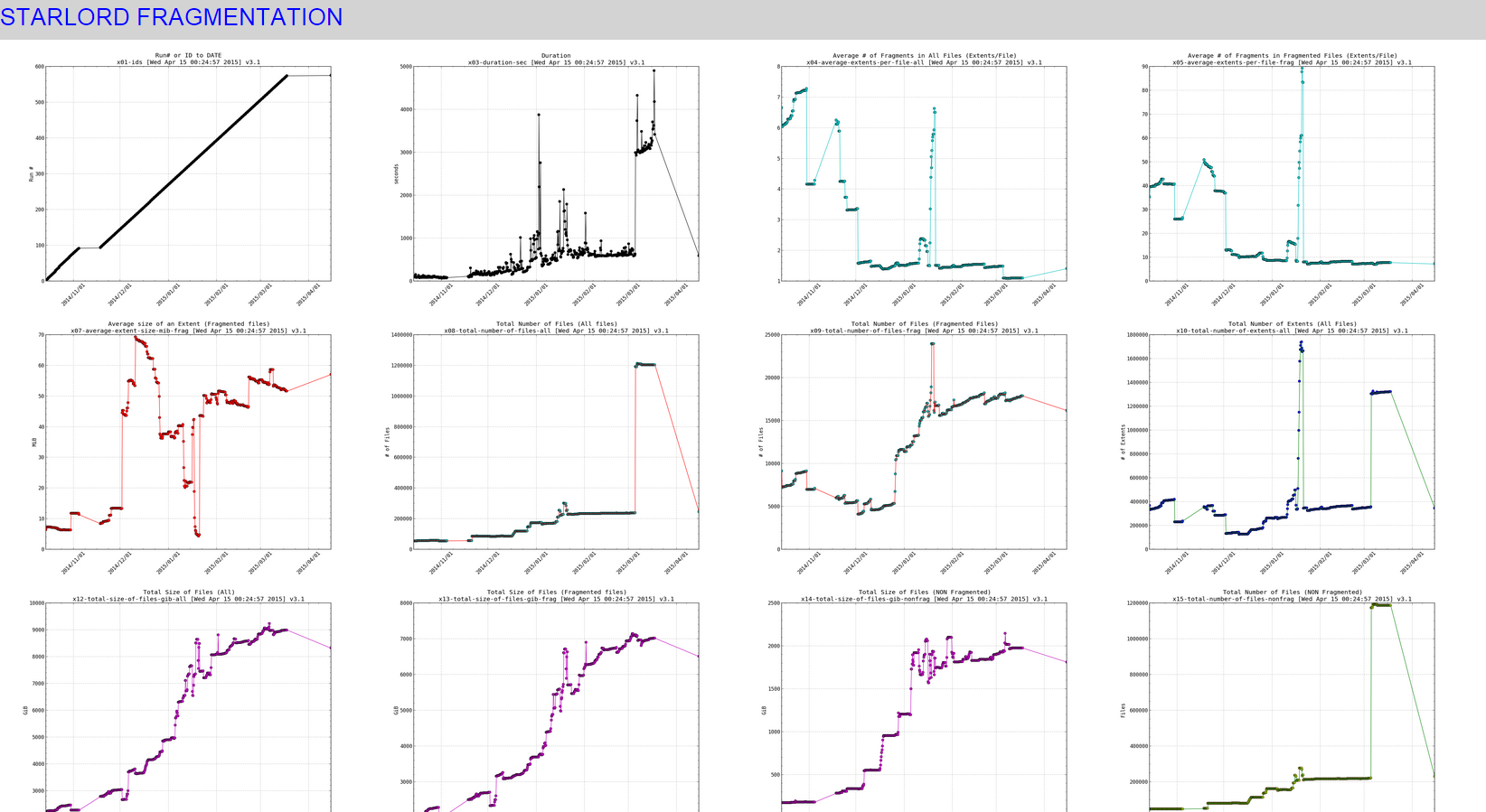
EXAMPLE 2 – plotting fragmentation
I generated data for these plotting scripts using a cron job that runs this mostfragged script over and over. Which measures fragmentation in my volume.
Here are examples of the plots (live): http://www.infotinks.com/fragplots/
DEADLINKS: http://www.infotinks.com/plot/ & http://www.infotinks.com/plotdk/
Snapshot of the small thumbnails:
When clicking on any of the pics (it would open a really high resolution image that you can zoom in on , to see effect click on the links above to see the live data):
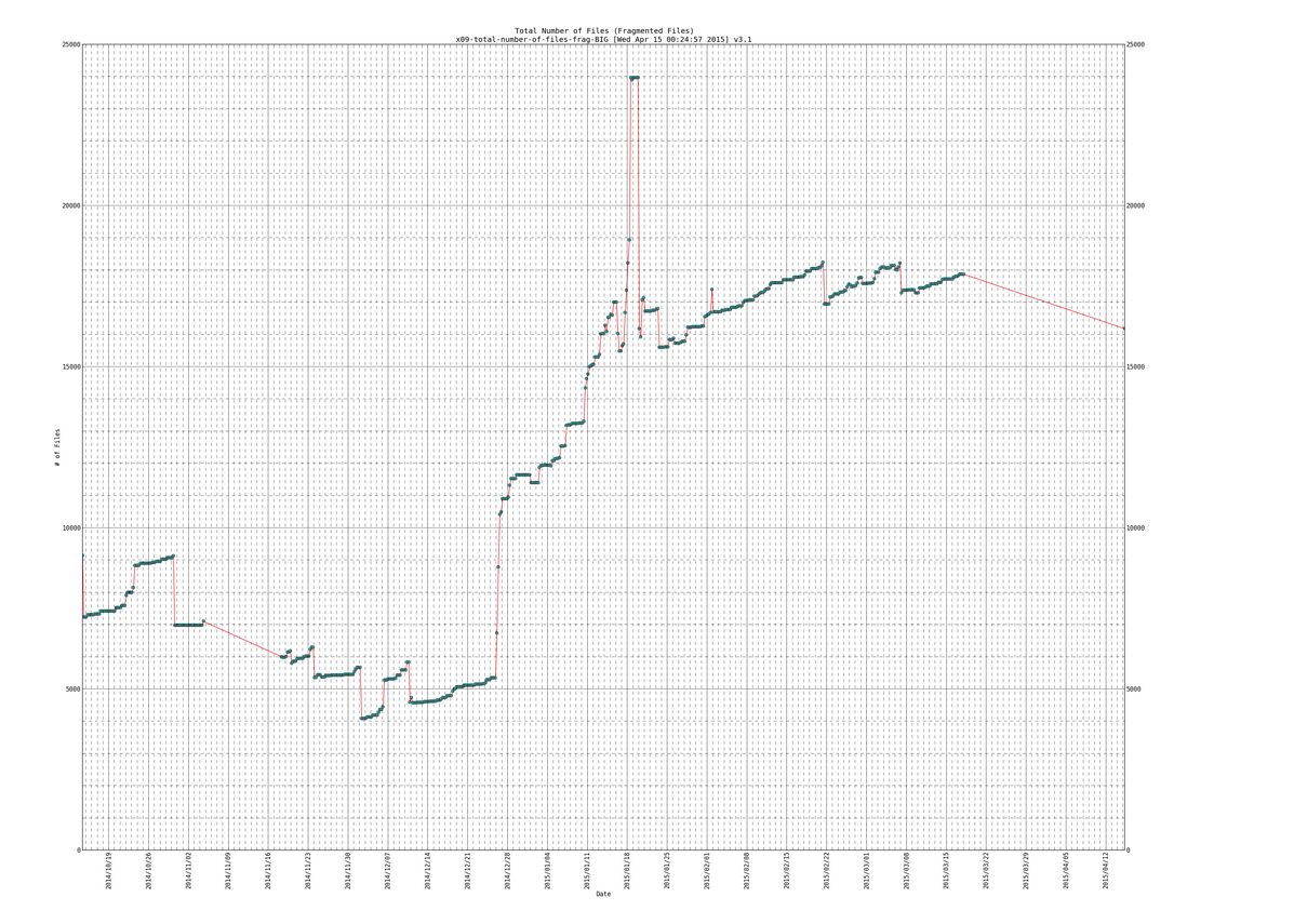
SIDENOTE: ignore the part in my plots where the line slopes downward at the end, thats due to the fragmentation scripts data gathering part not working for a while (a month or so) and then picking back up again.
Lines of data that we will be parsing:
   570  [Mon Mar 16 18:30:01 PDT 2015] DATEs|1426555801|DURs|3546|AVEXTENTS|1.09651/7.74861|AVSIZEmib|6.97168/52.0035|TOTFILES|1204209/17825|TOTEXTENTS|1320431/138119|TOTALSIZEgib|8989.86/7014.32 (All files/Fragmented files)
   571  [Tue Mar 17 00:30:01 PDT 2015] DATEs|1426577401|DURs|3623|AVEXTENTS|1.09737/7.79074|AVSIZEmib|6.96862/51.6225|TOTFILES|1204288/17868|TOTEXTENTS|1321553/139205|TOTALSIZEgib|8993.55/7017.69 (All files/Fragmented files)
   572  [Tue Mar 17 06:30:01 PDT 2015] DATEs|1426599001|DURs|4902|AVEXTENTS|1.09739/7.79176|AVSIZEmib|6.96905/51.6183|TOTFILES|1204289/17869|TOTEXTENTS|1321579/139231|TOTALSIZEgib|8994.29/7018.43 (All files/Fragmented files)
   573  [Tue Mar 17 12:30:01 PDT 2015] DATEs|1426620601|DURs|4180|AVEXTENTS|1.09739/7.79176|AVSIZEmib|6.96905/51.6183|TOTFILES|1204289/17869|TOTEXTENTS|1321579/139231|TOTALSIZEgib|8994.29/7018.43 (All files/Fragmented files)
   574  [Tue Mar 17 18:30:01 PDT 2015] DATEs|1426642201|DURs|3418|AVEXTENTS|1.09739/7.79176|AVSIZEmib|6.96904/51.6183|TOTFILES|1204291/17869|TOTEXTENTS|1321581/139231|TOTALSIZEgib|8994.29/7018.43 (All files/Fragmented files)
   575  [Wed Apr 15 00:15:02 PDT 2015] DATEs|1429082102|DURs|593|AVEXTENTS|1.4078/7.21457|AVSIZEmib|24.6336/57.065|TOTFILES|245616/16181|TOTEXTENTS|345777/116739|TOTALSIZEgib|8318.11/6505.58 (All files/Fragmented files)
Here is the fragmentation plotall.py:
#!/usr/bin/python
# filename: /root/docs/frag/plot/plotall.py
# how to run: /root/docs/frag/plot/plotall.py or /root/docs/frag/plot/plot-and-tx.sh

###############
### IMPORTS ###
###############

import re
import matplotlib as mb
mb.use('Agg')
import matplotlib.pyplot as plt
import matplotlib.dates as mdate
from matplotlib.dates import MO, TU, WE, TH, FR, SA, SU
import time
import numpy as np

############
### VARS ###
############

### input and output variables ###
DATAFILE='/root/docs/frag/table0.txt'
OUTPUTDIR='/root/docs/frag/plot/output/'
### title variables ###
VERSIONNUM="3.1"
TIMESTART=time.strftime("%c")
### error debuging ###
PRINT_DEBUG=1
PRINT_ERROR_DEBUG=1
### default font ###
DEFAULTFONT='Bitstream Vera Sans Mono'
### height and width of plots ###
WIDTH_SMALL=12 # 8x6 looks good
HEIGHT_SMALL=9
MAGNIFY=3
WIDTH_BIG=WIDTH_SMALL*MAGNIFY
HEIGHT_BIG=HEIGHT_SMALL*MAGNIFY

############
### DEFS ###
############

def drawit(x,y,colors1,filenamesave,goodtitle,yaxislabel="0",bigger=False,ymin=-1,ymax=-1):
    # set default font (for no warning)
    mb.rcParams['font.family'] = DEFAULTFONT
    # select main plot (which is same as sublot 1 of 1x1 = 111)
    # ax = plt.subplot(111)
    # clear old plots (so they dont stack up)
    plt.clf(); # clear figure
    plt.cla(); # clear axis
    # on big plots filename has extra suffix
    if bigger == True:
        filenamesave=filenamesave+"-BIG"
    # set title and y and xaxis stuff
    plt.title(goodtitle + '\n' + filenamesave + ' [' + TIMESTART + '] v' + VERSIONNUM)
    plt.xlabel('Date')
    # set y axis label, if yaxislabel is 0 then we leave y axis as default
    if yaxislabel == "0":
        pass
    else:
        plt.ylabel(yaxislabel) # set y axis label
    # enable simple grid (later we can define a better grid for "bigger" graphs)
    plt.grid()
    # rotate xticks 45 degrees
    plt.xticks( rotation=45 )
    # convert x axis dates (which are in unix epoch seconds) to numbers that matplotlib likes
    xmb=mdate.epoch2num(x)
    #### OPTIONAL::: formatting axis for dates
    #### plt.gca().autoscale_view()
    # plot minorticks_on for y axis
    plt.minorticks_on()
    if bigger == True:
        #### move title higher (no need anymore as not putting xticks on top)
        #### plt.title(goodtitle + '\n' + filenamesave + ' [' + TIMESTART + '] v' + VERSIONNUM, y=1.08)
        # on bigger graph we need to give more stuff to the x axis and get more grid lines (one minor for each day)
        # if bigger is not set (bigger = False) then just graph everything defaultly (it will autoscale everything)
        plt.xticks( rotation=90 )
        # use mdate to find marking points for x axis
        sundays=mdate.WeekdayLocator(byweekday=SU) # each SUNDAY gets a major gridline
        ####### dayformat=mdate.DateFormatter('%Y/%m/%d') # each SUNDAY thats marked on xaxis will get this date format ####### we do it below now
        days=mdate.DayLocator()
        # now mark the xaxis
        plt.gca().xaxis.set_major_locator(sundays) # mark sundays for major gridlines
        ####### plt.gca().xaxis.set_major_formatter(dayformat) ######### - we do it below now
        plt.gca().xaxis.set_minor_locator(days) # mark days for minor gridlines
        # get better/more grid lines for the bigger plot (now the minor grid gets lines as well)
        plt.grid(b=True,which='major',linestyle='-')
        plt.grid(b=True,which='minor',linestyle='--')
        # on bigger plots lets have more labels on axes
        #plt.gca().tick_params(labeltop=True, labelright=True)
        plt.gca().tick_params(labelright=True)
        # rotate top ticks
        #for tick in plt.gca().get_xticklabels():
        #    tick.set_rotation(90)
    dayformat=mdate.DateFormatter('%Y/%m/%d') # each SUNDAY thats marked on xaxis will get this date format
    plt.gca().xaxis.set_major_formatter(dayformat)
    # setting ymin and ymax for yaxis if ymin is not -1 and ymax is not -1
    dg("* %s y limit [%s, %s]" % (str(filenamesave),str(ymin),str(ymax)))
    if (not (ymin == -1) and not (ymax == -1)):
        dg("    Changing yaxis min and max on %s to [%s, %s]" % (str(filenamesave),str(ymin),str(ymax)))
        plt.gca().set_ylim([ymin,ymax])
    # they stack up (which is good as they are the same plot
    plt.plot_date(xmb,y,colors1[0]) # plot the line with first set of colors (could be a circle)
    plt.plot_date(xmb,y,colors1[1]) # plot the same line with second set of colors  (could be a line this time)
    # set size of main figure
    optionalbigtext=''
    fig = mb.pyplot.gcf()
    if bigger == True:
        FINAL_WIDTH=WIDTH_BIG
        FINAL_HEIGHT=HEIGHT_BIG
        optionalbigtext='big'
    else:
        FINAL_WIDTH=WIDTH_SMALL
        FINAL_HEIGHT=HEIGHT_SMALL
        optionalbigtext='\b' #backspace so we dont get an extra space on the print statement
    # set size of figure
    fig.set_size_inches(FINAL_WIDTH,FINAL_HEIGHT)
    # save

    # directory /root/docs/frag/output should exist
    plt.savefig(OUTPUTDIR + filenamesave) # this appends .png because of the 'Agg' at the top
    print "Drew %s plot (%sin x %sin) '%s' to '%s'" % (optionalbigtext,FINAL_WIDTH,FINAL_HEIGHT,goodtitle,filenamesave + '.png')

## def drawit(x,y,colors1,filenamesave,goodtitle,yaxislabel="0"):
##    plt.clf();
##    plt.cla();
##    plt.title(goodtitle + '\n' + filenamesave + ' [' + TIMESTART + '] v' + VERSIONNUM)
##    plt.xlabel('Date&Time (unix epoch seconds)')
##    if yaxislabel =="0":
##        pass
##    else:
##        plt.ylabel(yaxislabel) # If need Y axis information
##    plt.grid()
##    plt.plot(x,y,colors1[0],x,y,colors1[1])
##    plt.savefig(OUTPUTDIR + filenamesave) # this appends .png because of the 'Agg' at the top
##    plt.savefig('/root/docs/frag/plot/output/' + filenamesave) # this appends .png because of the 'Agg' at the top
##    print "Drew '%s' to '%s'" % (goodtitle,filenamesave + '.png')

# dg is debug printing for developer debug messages
def dg(msg):
    # if PRINT_DEBUG is 1 then print the debug messages otherwise dont
    if PRINT_DEBUG == 1:
        print msg.rstrip('\n') # we strip the last empty line that might exist

# dge is debug printing for errors
def dge(msg):
    # if PRINT_ERROR_DEBUG is 1 then print the debug messages otherwise dont
    if PRINT_ERROR_DEBUG == 1:
        print msg.rstrip('\n') # we strip the last empty line that might exist

############
### MAIN ###
############

# file /root/docs/frag/table0.txt should exist and have the data that cron.sh generates daily (4 times daily, or however many time)
f=open(DATAFILE,'r')
num=0
x1,x2,x3,x4,x5,x6,x7,x8,x9,x10,x11,x12,x13,x14,x15,x16=[],[],[],[],[],[],[],[],[],[],[],[],[],[],[],[];
# adding new one
x17=[]
x18=[]
x19=[]
x20=[]
for line in f:
    # a line is a row. num is line number (starting at 1 for first line)
    num+=1
    orgline=line
    linenoparenthesis=re.split('\(',orgline)
    barsplit=re.split('[\||/]',linenoparenthesis[0]) # split by | and /
    # cnum is chunk number (starting at 1 for first chunk)
    cnum=0
    dg("~~~~~~~~~~~~~~~~~~~~~~~~~~~~~~~~~~~~~~~~~~~~~~~~~~~~~~~~~~~~~~~~~~~~~~~~~~~~~~~~~~~~~~~~")
    dg(line)
    did_x1=0
    did_x2=0
    did_x3=0
    did_x4=0
    did_x5=0
    did_x6=0
    did_x7=0
    did_x8=0
    did_x9=0
    did_x10=0
    did_x11=0
    did_x12=0
    did_x13=0
    did_x14=0
    did_x15=0
    did_x16=0
    did_x17=0
    did_x18=0
    did_x19=0
    did_x20=0
    try:
        # a chunk is a column in the line
        for chunk in barsplit:
            cnum+=1
            if cnum==1:
                n1fragnum=float(re.split('\[',chunk)[0].strip()); # fragmentation run number (iteration number)
                x1.append(n1fragnum)
                dg("    chunk #{0}: {1}".format(str(cnum),str(n1fragnum)))
                did_x1=1
            elif cnum==2:
                n2date=float(chunk); # date in seconds (epoch)
                x2.append(n2date)
                dg("    chunk #{0}: {1}".format(str(cnum),str(n2date)))
                did_x2=1
            elif cnum==4:
                n3duration=float(chunk); # duration of the whole run in seconds
                x3.append(n3duration)
                dg("    chunk #{0}: {1}".format(str(cnum),str(n3duration)))
                did_x3=1
            elif cnum==6:
                n4avextall=float(chunk); # average num of extents in a file (all files)
                x4.append(n4avextall)
                dg("    chunk #{0}: {1}".format(str(cnum),str(n4avextall)))
                did_x4=1
            elif cnum==7:
                n5avextfrag=float(chunk); # average num of extents in a file (fragged files)
                x5.append(n5avextfrag)
                dg("    chunk #{0}: {1}".format(str(cnum),str(n5avextfrag)))
                did_x5=1
            elif cnum==9:
                n6avsizemiball=float(chunk); # average size of an extent in a file (all files) (MiB)
                x6.append(n6avsizemiball)
                dg("    chunk #{0}: {1}".format(str(cnum),str(n6avsizemiball)))
                did_x6=1
            elif cnum==10:
                n7avsizemibfrag=float(chunk); # average size of an extent in a file (fragged files) (MiB)
                x7.append(n7avsizemibfrag)
                dg("    chunk #{0}: {1}".format(str(cnum),str(n7avsizemibfrag)))
                did_x7=1
            elif cnum==12:
                n8totfilesall=float(chunk); # total number of files (all files)
                x8.append(n8totfilesall)
                dg("    chunk #{0}: {1}".format(str(cnum),str(n8totfilesall)))
                did_x8=1
            elif cnum==13:
                n9totfilesfrag=float(chunk); # total number of files (fragged)
                x9.append(n9totfilesfrag)
                dg("    chunk #{0}: {1}".format(str(cnum),str(n9totfilesfrag)))
                did_x9=1
            elif cnum==15:
                n10totextall=float(chunk); # total number of extents (all files)
                x10.append(n10totextall)
                dg("    chunk #{0}: {1}".format(str(cnum),str(n10totextall)))
                did_x10=1
            elif cnum==16:
                n11totextfrag=float(chunk); # total number of extents (fragged files)
                x11.append(n11totextfrag)
                dg("    chunk #{0}: {1}".format(str(cnum),str(n11totextfrag)))
                did_x11=1
            elif cnum==18:
                n12totsizegiball=float(chunk); # size of all files combined (should be close to disk used) (GiB)
                x12.append(n12totsizegiball)
                dg("    chunk #{0}: {1}".format(str(cnum),str(n12totsizegiball)))
                did_x12=1
            elif cnum==19:
                n13totsizegibfrag=float(chunk); # size of all fragged files combined (GiB)
                x13.append(n13totsizegibfrag)
                dg("    chunk #{0}: {1}".format(str(cnum),str(n13totsizegibfrag)))
                did_x13=1
        # calc new numbers not in table
        n14totsizenonefraggedfiles=n12totsizegiball-n13totsizegibfrag #total size of unfragmented files (0 or 1 extent) (GiB)
        n15totfilesnonefragged=n8totfilesall-n9totfilesfrag #total number of unfraggmented files (0 or 1 extent)
        n16totextsnonefragged=n10totextall-n11totextfrag #total number of unfrag extents (0 or 1 extents)
        # new
        n17percentfragmentationbyfile=(float(n9totfilesfrag)/float(n8totfilesall))*100.0
        n18percentfragmentationbyext=(float(n11totextfrag)/float(n10totextall))*100.0
        n19percentfragmentationbysize=(float(n13totsizegibfrag)/float(n12totsizegiball))*100.0
        n20percentfragaverage=(n17percentfragmentationbyfile + n18percentfragmentationbyext + n19percentfragmentationbysize)/3.0
        # add new numbers to x
        x14.append(n14totsizenonefraggedfiles)
        dg("    chunk #{0}: {1}".format(str(cnum),str(n14totsizenonefraggedfiles)))
        did_x14=1
        x15.append(n15totfilesnonefragged)
        dg("    chunk #{0}: {1}".format(str(cnum),str(n15totfilesnonefragged)))
        did_x15=1
        x16.append(n16totextsnonefragged)
        dg("    chunk #{0}: {1}".format(str(cnum),str(n16totextsnonefragged)))
        did_x16=1
        # new
        x17.append(n17percentfragmentationbyfile)
        dg("    chunk #{0}: {1}".format(str(cnum),str(n17percentfragmentationbyfile)))
        did_x17=1
        x18.append(n18percentfragmentationbyext)
        dg("    chunk #{0}: {1}".format(str(cnum),str(n18percentfragmentationbyext)))
        did_x18=1
        x19.append(n19percentfragmentationbysize)
        dg("    chunk #{0}: {1}".format(str(cnum),str(n19percentfragmentationbysize)))
        did_x19=1
        x20.append(n20percentfragaverage)
        dg("    chunk #{0}: {1}".format(str(cnum),str(n20percentfragaverage)))
        did_x20=1
    except ValueError as e:
        # if error occured before whole line was processed we need to undo any inserts that we did for that line, and continue to next line.
        dge("* ERROR ON THIS LINE: {0}".format(line))
        dge("* did_x1: {0} {1}".format(str(did_x1),len(x1)))
        dge("* did_x2: {0} {1}".format(str(did_x2),len(x2)))
        dge("* did_x3: {0} {1}".format(str(did_x3),len(x3)))
        dge("* did_x4: {0} {1}".format(str(did_x4),len(x4)))
        dge("* did_x5: {0} {1}".format(str(did_x5),len(x5)))
        dge("* did_x6: {0} {1}".format(str(did_x6),len(x6)))
        dge("* did_x7: {0} {1}".format(str(did_x7),len(x7)))
        dge("* did_x8: {0} {1}".format(str(did_x8),len(x8)))
        dge("* did_x9: {0} {1}".format(str(did_x9),len(x9)))
        dge("* did_x10: {0} {1}".format(str(did_x10),len(x10)))
        dge("* did_x11: {0} {1}".format(str(did_x11),len(x11)))
        dge("* did_x12: {0} {1}".format(str(did_x12),len(x12)))
        dge("* did_x13: {0} {1}".format(str(did_x13),len(x13)))
        dge("* did_x14: {0} {1}".format(str(did_x14),len(x14)))
        dge("* did_x15: {0} {1}".format(str(did_x15),len(x15)))
        dge("* did_x16: {0} {1}".format(str(did_x16),len(x16)))
        dge("* did_x17: {0} {1}".format(str(did_x17),len(x17)))
        dge("* did_x18: {0} {1}".format(str(did_x18),len(x18)))
        dge("* did_x19: {0} {1}".format(str(did_x19),len(x19)))
        dge("* did_x20: {0} {1}".format(str(did_x20),len(x20)))
        if did_x1 == 1:
            x1.pop()
        if did_x2 == 1:
            x2.pop()
        if did_x3 == 1:
            x3.pop()
        if did_x4 == 1:
            x4.pop()
        if did_x5 == 1:
            x5.pop()
        if did_x6 == 1:
            x6.pop()
        if did_x7 == 1:
            x7.pop()
        if did_x8 == 1:
            x8.pop()
        if did_x9 == 1:
            x9.pop()
        if did_x10 == 1:
            x10.pop()
        if did_x11 == 1:
            x11.pop()
        if did_x12 == 1:
            x12.pop()
        if did_x13 == 1:
            x13.pop()
        if did_x14 == 1:
            x14.pop()
        if did_x15 == 1:
            x15.pop()
        if did_x16 == 1:
            x16.pop()
        if did_x17 == 1:
            x17.pop()
        if did_x18 == 1:
            x18.pop()
        if did_x19 == 1:
            x19.pop()
        if did_x20 == 1:
            x20.pop()
        dge("* did_x1: after {0}".format(len(x1)))
        dge("* did_x2: after {0}".format(len(x2)))
        dge("* did_x3: after {0}".format(len(x3)))
        dge("* did_x4: after {0}".format(len(x4)))
        dge("* did_x5: after {0}".format(len(x5)))
        dge("* did_x6: after {0}".format(len(x6)))
        dge("* did_x7: after {0}".format(len(x7)))
        dge("* did_x8: after {0}".format(len(x8)))
        dge("* did_x9: after {0}".format(len(x9)))
        dge("* did_x10: after {0}".format(len(x10)))
        dge("* did_x11: after {0}".format(len(x11)))
        dge("* did_x12: after {0}".format(len(x12)))
        dge("* did_x13: after {0}".format(len(x13)))
        dge("* did_x14: after {0}".format(len(x14)))
        dge("* did_x15: after {0}".format(len(x15)))
        dge("* did_x16: after {0}".format(len(x16)))
        dge("* did_x17: after {0}".format(len(x17)))
        dge("* did_x18: after {0}".format(len(x18)))
        dge("* did_x19: after {0}".format(len(x19)))
        dge("* did_x20: after {0}".format(len(x20)))
        continue
    dg( '%f,%f,%f,%f,%f,%f,%f,%f,%f,%f,%f,%f,%f,%f,%f,%f,%f,%f,%f,%f,%f' % \
            (n1fragnum,n2date,n3duration,n4avextall,n5avextfrag,n6avsizemiball,n7avsizemibfrag,n8totfilesall,
                    n9totfilesfrag,n10totextall,n11totextfrag,n12totsizegiball,n13totsizegibfrag,n14totsizenonefraggedfiles,
                    n14totsizenonefraggedfiles,n15totfilesnonefragged,n16totextsnonefragged,n17percentfragmentationbyfile,n18percentfragmentationbyext,n19percentfragmentationbysize,n20percentfragaverage) )
f.close()
dg("~~~~~~~~~~~~~~~~~~~~~~~~~~~~~~~~~~~~~~~~~~~~~~~~~~~~~~~~~~~~~~~~~~~~~~~~~~~~~~~~~~~~~~~~")
print 'Done Parsing, Starting To Make Drawings'
# graph plots, that are split into groups (each group has the same colors) #
# --- group 1 --- #
drawit(x2,x1,['ko','k'],"x01-ids","Run# or ID to DATE",yaxislabel="Run #")
drawit(x2,x3,['ko','k'],"x03-duration-sec","Duration",yaxislabel="seconds")
drawit(x2,x1,['ko','k'],"x01-ids","Run# or ID to DATE",yaxislabel="Run #",bigger=True)
drawit(x2,x3,['ko','k'],"x03-duration-sec","Duration",yaxislabel="seconds",bigger=True)
# --- group 2 --- #
drawit(x2,x4,['co','c'],"x04-average-extents-per-file-all","Average # of Fragments in All Files (Extents/File)")
drawit(x2,x5,['co','c'],"x05-average-extents-per-file-frag","Average # of Fragments in Fragmented Files (Extents/File)")
drawit(x2,x4,['co','c'],"x04-average-extents-per-file-all","Average # of Fragments in All Files (Extents/File)",bigger=True)
drawit(x2,x5,['co','c'],"x05-average-extents-per-file-frag","Average # of Fragments in Fragmented Files (Extents/File)",bigger=True)
# --- group 3 --- #
drawit(x2,x6,['ro','r'],"x06-average-extent-size-mib-all","Average size of an Extents (All files)",yaxislabel="MiB")
drawit(x2,x7,['ro','r'],"x07-average-extent-size-mib-frag","Average size of an Extent (Fragmented files)",yaxislabel="MiB")
drawit(x2,x6,['ro','r'],"x06-average-extent-size-mib-all","Average size of an Extents (All files)",yaxislabel="MiB",bigger=True)
drawit(x2,x7,['ro','r'],"x07-average-extent-size-mib-frag","Average size of an Extent (Fragmented files)",yaxislabel="MiB",bigger=True)
# --- group 4 --- #
drawit(x2,x8,['co','r'],"x08-total-number-of-files-all","Total Number of Files (All files)",yaxislabel="# of Files")
drawit(x2,x9,['co','r'],"x09-total-number-of-files-frag","Total Number of Files (Fragmented Files)",yaxislabel="# of Files")
drawit(x2,x8,['co','r'],"x08-total-number-of-files-all","Total Number of Files (All files)",yaxislabel="# of Files",bigger=True)
drawit(x2,x9,['co','r'],"x09-total-number-of-files-frag","Total Number of Files (Fragmented Files)",yaxislabel="# of Files",bigger=True)
# --- group 5 --- #
drawit(x2,x10,['bo','g'],"x10-total-number-of-extents-all","Total Number of Extents (All Files)",yaxislabel="# of Extents")
drawit(x2,x11,['bo','g'],"x11-total-number-of-extents-frag","Total Number of Extents (Fragmented Files)",yaxislabel="# of Extents")
drawit(x2,x10,['bo','g'],"x10-total-number-of-extents-all","Total Number of Extents (All Files)",yaxislabel="# of Extents",bigger=True)
drawit(x2,x11,['bo','g'],"x11-total-number-of-extents-frag","Total Number of Extents (Fragmented Files)",yaxislabel="# of Extents",bigger=True)
# --- group 6 --- #
drawit(x2,x12,['mo','m'],"x12-total-size-of-files-gib-all","Total Size of Files (All)",yaxislabel="GiB")
drawit(x2,x13,['mo','m'],"x13-total-size-of-files-gib-frag","Total Size of Files (Fragmented files)",yaxislabel="GiB")
drawit(x2,x14,['mo','m'],"x14-total-size-of-files-gib-nonfrag","Total Size of Files (NON Fragmented)",yaxislabel="GiB")
drawit(x2,x12,['mo','m'],"x12-total-size-of-files-gib-all","Total Size of Files (All)",yaxislabel="GiB",bigger=True)
drawit(x2,x13,['mo','m'],"x13-total-size-of-files-gib-frag","Total Size of Files (Fragmented files)",yaxislabel="GiB",bigger=True)
drawit(x2,x14,['mo','m'],"x14-total-size-of-files-gib-nonfrag","Total Size of Files (NON Fragmented)",yaxislabel="GiB",bigger=True)
# --- group 7 --- #
drawit(x2,x15,['yo','g'],"x15-total-number-of-files-nonfrag","Total Number of Files (NON Fragmented)",yaxislabel="Files")
drawit(x2,x16,['yo','g'],"x16-total-number-of-extents-nonfrag","Total Number of Extents (NON Fragmented)",yaxislabel="Extents")
drawit(x2,x15,['yo','g'],"x15-total-number-of-files-nonfrag","Total Number of Files (NON Fragmented)",yaxislabel="Files",bigger=True)
drawit(x2,x16,['yo','g'],"x16-total-number-of-extents-nonfrag","Total Number of Extents (NON Fragmented)",yaxislabel="Extents",bigger=True)
# --- new group 8 --- #
drawit(x2,x17,['ko','r'],"x17-percent-frag-by-files","Percent Fragmentation (# of Fragmented Files / All Files)",yaxislabel="%",ymin=0,ymax=100)
drawit(x2,x18,['ko','r'],"x18-percent-frag-by-extents","Percent Fragmentation (# of Fragmented Extents / All Extents)",yaxislabel="%",ymin=0,ymax=100)
drawit(x2,x19,['ko','r'],"x19-percent-frag-by-size","Percent Fragmentation (# of Fragmented MiB / All MiB)",yaxislabel="%",ymin=0,ymax=100)
drawit(x2,x20,['ko','r'],"x20-percent-frag-average","Percent Fragmentation Average of the Above",yaxislabel="%",ymin=0,ymax=100)
drawit(x2,x17,['ko','r'],"x17-percent-frag-by-files","Percent Fragmentation (# of Fragmented Files / All Files)",yaxislabel="%",bigger=True,ymin=0,ymax=100)
drawit(x2,x18,['ko','r'],"x18-percent-frag-by-extents","Percent Fragmentation (# of Fragmented Extents / All Extents)",yaxislabel="%",bigger=True,ymin=0,ymax=100)
drawit(x2,x19,['ko','r'],"x19-percent-frag-by-size","Percent Fragmentation (# of Fragmented MiB / All MiB)",yaxislabel="%",bigger=True,ymin=0,ymax=100)
drawit(x2,x20,['ko','r'],"x20-percent-frag-average","Percent Fragmentation Average of the Above",yaxislabel="%",bigger=True,ymin=0,ymax=100)
Here is the fragmentation index.html
<!DOCTYPE HTML>
<html>
<meta http-equiv="Content-Type" content="text/html; charset=UTF-8"/>
<title>STARLORD FRAGMENTATION</title>
<link rel="stylesheet" href="https://maxcdn.bootstrapcdn.com/bootstrap/3.3.0/css/bootstrap.min.css">
<style>
  body {background-color:lightgray}
  h3   {color:blue}
  p    {color:green}
  img  {width:370px;height:270px;border:1;}
</style>
</head>
<section>
<h3>STARLORD FRAGMENTATION</h3>
<!--
ALL FILES: These are the files, for each one there is a bigger plot with BIG suffix in the filename
x01-ids.png
x03-duration-sec.png
x04-average-extents-per-file-all.png
x05-average-extents-per-file-frag.png
x06-average-extent-size-mib-all.png
x07-average-extent-size-mib-frag.png
x08-total-number-of-files-all.png
x09-total-number-of-files-frag.png
x10-total-number-of-extents-all.png
x11-total-number-of-extents-frag.png
x12-total-size-of-files-gib-all.png
x13-total-size-of-files-gib-frag.png
x14-total-size-of-files-gib-nonfrag.png
x15-total-number-of-files-nonfrag.png
x16-total-number-of-extents-nonfrag.png
x17-percent-frag-by-files.png
x18-percent-frag-by-extents.png
x19-percent-frag-by-size.png
x20-percent-frag-average.png
-->
<table style="width:100%">
  <tr>
    <td><a href="x01-ids-BIG.png"><img src="x01-ids.png"></a></td>
    <td><a href="x03-duration-sec-BIG.png"><img src="x03-duration-sec.png"></a></td>
    <td><a href="x04-average-extents-per-file-all-BIG.png"><img src="x04-average-extents-per-file-all.png"></a></td>
    <td><a href="x05-average-extents-per-file-frag-BIG.png"><img src="x05-average-extents-per-file-frag.png"></a></td>
    <td><a href="x06-average-extent-size-mib-all-BIG.png"><img src="x06-average-extent-size-mib-all.png"></a></td>
  </tr>
  <tr>
    <td><a href="x07-average-extent-size-mib-frag-BIG.png"><img src="x07-average-extent-size-mib-frag.png"></a></td>
    <td><a href="x08-total-number-of-files-all-BIG.png"><img src="x08-total-number-of-files-all.png"></a></td>
    <td><a href="x09-total-number-of-files-frag-BIG.png"><img src="x09-total-number-of-files-frag.png"></a></td>
    <td><a href="x10-total-number-of-extents-all-BIG.png"><img src="x10-total-number-of-extents-all.png"></a></td>
    <td><a href="x11-total-number-of-extents-frag-BIG.png"><img src="x11-total-number-of-extents-frag.png"></a></td>
  </tr>
  <tr>
    <td><a href="x12-total-size-of-files-gib-all-BIG.png"><img src="x12-total-size-of-files-gib-all.png"></a></td>
    <td><a href="x13-total-size-of-files-gib-frag-BIG.png"><img src="x13-total-size-of-files-gib-frag.png"></a></td>
    <td><a href="x14-total-size-of-files-gib-nonfrag-BIG.png"><img src="x14-total-size-of-files-gib-nonfrag.png"></a></td>
    <td><a href="x15-total-number-of-files-nonfrag-BIG.png"><img src="x15-total-number-of-files-nonfrag.png"></a></td>
    <td><a href="x16-total-number-of-extents-nonfrag-BIG.png"><img src="x16-total-number-of-extents-nonfrag.png"></a></td>
  </tr>
  <tr>
    <td><a href="x17-percent-frag-by-files-BIG.png"><img src="x17-percent-frag-by-files.png"></a></td>
    <td><a href="x18-percent-frag-by-extents-BIG.png"><img src="x18-percent-frag-by-extents.png"></a></td>
    <td><a href="x19-percent-frag-by-size-BIG.png"><img src="x19-percent-frag-by-size.png"></a></td>
    <td><a href="x20-percent-frag-average-BIG.png"><img src="x20-percent-frag-average.png"></a></td>
  </tr>
</table>
</section>
<footer>
<p>Copyright 2012 - 2022 infotinks</p>
</footer>
</body>
</html>
EXAMPLE 3 – transfer rates on my iptest server
SIDENOTE: This example has Trend line, so if you want to see that look for the section of code that start with “TRENDLINE” and ends with “TRENDLINE end” (there should be 3 sections like that)
Here is the output (live):
DEADLINK: http://www.infotinks.com/c2strp/
Here is a snapshot of the small plots:
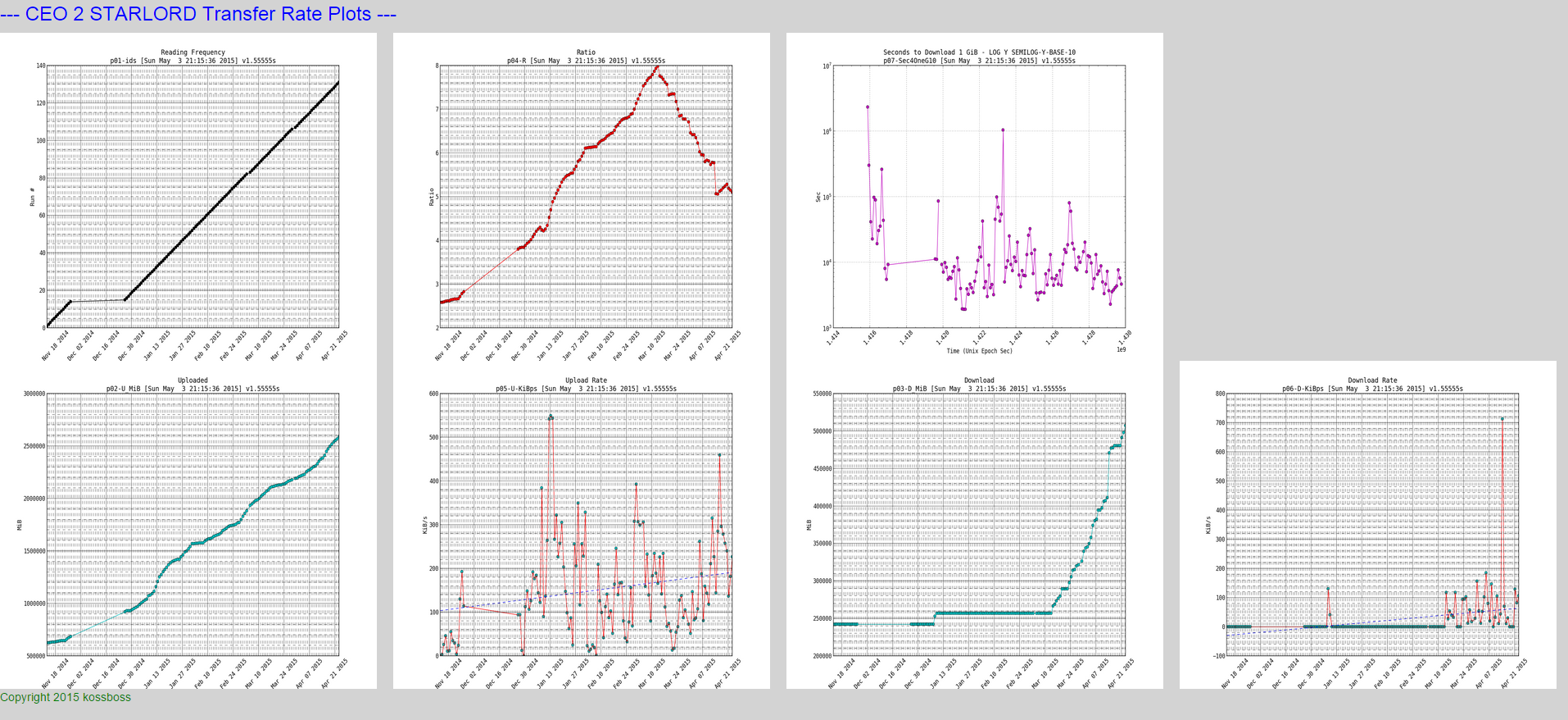
NOTE: if you look closely at the download and upload rates you can see a trend line which I will show how to plot in the python script
Here is a snapshot of the big plots:
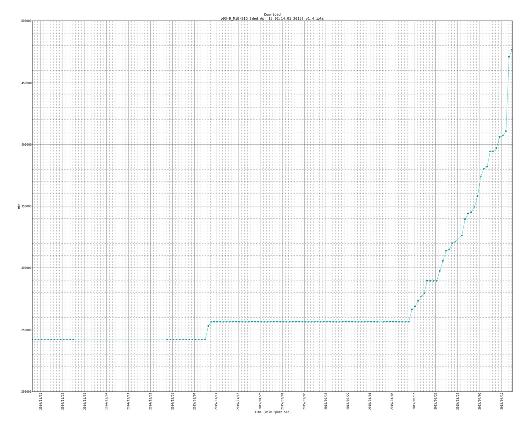
Here is an example of the big plot with the trend line (notice the version number is newer than plot above and it has more data entries as this one is newer than the plot directly above):
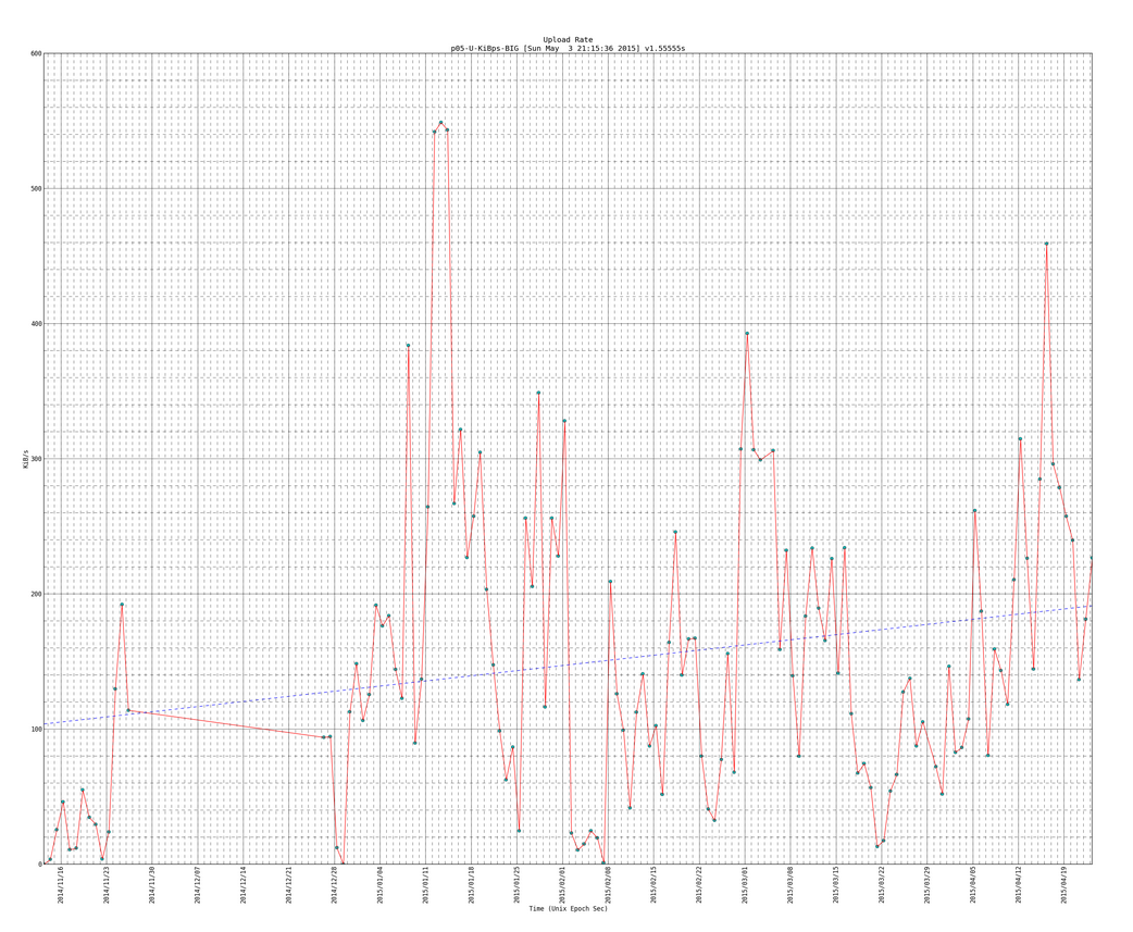
SIDENOTE: you will see code for trendlines, which I borrowed from here: http://widu.tumblr.com/post/43624347354/matplotlib-trendline which use the polyfit and poly1d functions (discussed more here: http://www.mathworks.com/help/matlab/ref/polyfit.html and http://docs.scipy.org/doc/numpy/reference/generated/numpy.poly1d.html )
Here is the data that we parsed:
* 121|Mon Apr 13 00:10:03 PDT 2015|1428909003|u 2.264tb 2489124696790b|d 401.189gb 430773116331b|r 5.77827|td 86399|ud 18.6483 GiB|dd 3.56251 GiB|226.324 ukps|43.2362 dkps|-0.00487006 rpd|-0.146102 rpm|-1.77757 rpy|4633.07s/g|01:17:13/g
* 122|Tue Apr 14 00:10:03 PDT 2015|1428995403|u 2.275tb 2501896013710b|d 459.911gb 493825464267b|r 5.06636|td 86400|ud 11.8942 GiB|dd 58.722 GiB|144.352 ukps|712.668 dkps|-0.71191 rpd|-21.3573 rpm|-259.847 rpy|7264.02s/g|02:01:04/g
* 123|Wed Apr 15 00:10:02 PDT 2015|1429081802|u 2.298tb 2527122353386b|d 465.665gb 500003634891b|r 5.05421|td 86399|ud 23.4938 GiB|dd 5.75387 GiB|285.131 ukps|69.8315 dkps|-0.0121501 rpd|-0.364504 rpm|-4.4348 rpy|3677.52s/g|01:01:17/g
* 124|Wed Apr 15 02:10:03 PDT 2015|1429089003|u 2.299tb 2528123299301b|d 465.665gb 500003634891b|r 5.05621|td 7201|ud 954.576 MiB|dd 0 B|135.743 ukps|0 dkps|0.0239967 rpd|0.7199 rpm|8.75878 rpy|7724.72s/g|02:08:44/g
Here is the script:
#!/usr/bin/python
# filename: /root/scripts/ipt/plotall.py
# how to run: /root/scripts/ipt/plotall.py
# ipt folder is where everything is including this script it has my Inter Personal server Transfer rates
# *** if your interested in TREND LINES then look for "TRENDLINE CODE:" where the trend line code starts, and "end of TRENDLINE CODE" where the trendline code ends (there should be 3 sections of that)

############################
### LIBRARY IMPORT LINES ###
############################

import re
import matplotlib as mb
mb.use('Agg')
import matplotlib.pyplot as plt
import matplotlib.dates as mdate
from matplotlib.dates import MO, TU, WE, TH, FR, SA, SU
import time
# TRENDLINE uses numpy
import numpy as np
# end of TRENDLINE CODE

#################
### VARIABLES ###
#################

# get Versions and time for title
VERSIONNUM="1.7"
TIMESTART=time.strftime("%c")
# output directory for plots and input file which has the input data
OUTPUTDIR="/root/scripts/ipt/plots/"
# can pick any of these:
##/root/scripts/ipt/analysis/analysis-1-hourly.txt
##/root/scripts/ipt/analysis/analysis-12-hours.txt
##/root/scripts/ipt/analysis/analysis-24-daily.txt
##/root/scripts/ipt/analysis/analysis-from-first-to-last.txt
DATAFILE="/root/scripts/ipt/analysis/analysis-24-daily.txt"
# each line in the DATAFILE looks like this
# * 1482|Wed Feb 11 19:10:02 PST 2015|1423710602|u 1.547tb 1700684685540b|d 250.627gb 269108782443b|r 6.31969|td 3599|ud 622.438 MiB|dd 0 B|177.098 ukps|0 dkps|0.0580961 rpd|1.74288 rpm|21.2051 rpy|5920.88s/g|01:38:40/g
### BASE_Y_OF_LOGPLOT=10 - now its in argument
# DEFAULTFONT leave it be
DEFAULTFONT='Bitstream Vera Sans Mono'
# VARIABLES TO PRINT DEBUG MESSAGES OR NOT (1 print, 0 dont print)
PRINT_DEBUG=1
PRINT_ERROR_DEBUG=1
# HEIGHT and WIDTH
WIDTH_SMALL=12 # 8x6 looks good
HEIGHT_SMALL=9
MAGNIFY=3
WIDTH_BIG=WIDTH_SMALL*MAGNIFY
HEIGHT_BIG=HEIGHT_SMALL*MAGNIFY
#WIDTH_BIG=18.5*MAGNIFY
#HEIGHT_BIG=10.5*MAGNIFY
# TRENDLINE CODE: Trend degree, 1 is a line trendline (most common type of trendline), 2 is a curved line (x^2 type), 3 is x^3 line, the more the degree the more curves we will have - 4 is a good number, 3+ seem to all look alike as that is probably the best possible trendline. is you put 100 you might get errors, just keep that number between 1 inclusive and 10 inclusive
# numbers above 6 tend to get RankWarning warnings, which basically means the trendline is not the best it can be (lowering TRENDDEGREE is one way to fix it, the other way to fix it involves more code which I dont want to put in)
TRENDDEGREE=4
# note we didnt really need to have a full section for this, its just conventional to put code at the top
# end of TRENDLINE CODE (more below)

##################################
### DEBUG FUNCTIONS THAT PRINT ###
##################################

# dg is debug printing for developer debug messages
def dg(msg):
    # if PRINT_DEBUG is 1 then print the debug messages otherwise dont
    if PRINT_DEBUG == 1:
        print msg.rstrip('\n') # we strip the last empty line that might exist

# dge is debug printing for errors
def dge(msg):
    # if PRINT_ERROR_DEBUG is 1 then print the debug messages otherwise dont
    if PRINT_ERROR_DEBUG == 1:
        print msg.rstrip('\n') # we strip the last empty line that might exist

########################
### PLOTING FUNCTION ###
########################

def drawit(x,y,colors1,filenamesave,goodtitle,yaxislabel="0",logy="0",bigger="0",trend=False):
    # logy is 0 is regular plot, logy 2 is base2 semilog y plot, logy 10 is base 10 semilog y plot. put it in quotes
    # set font to not get font error (versa is on all pc) - or else get WARNING during run
    mb.rcParams['font.family'] = DEFAULTFONT
    # trying with selecting 1 subplot in 1x1 (so no subplots) - selecting current subplot
    ax = plt.subplot(111)
    # clear plot - or else plots stack up on top of each other
    plt.clf(); # clear figure
    plt.cla(); # clear axis
    # if bigger need to say so
    if bigger == "1":
        filenamesave=filenamesave+"-BIG"
    print "* DRAWING %s " % (filenamesave + '.png')
    # set title and y and xaxis stuff
    plt.title(goodtitle + '\n' + filenamesave + ' [' + TIMESTART + '] v' + VERSIONNUM)
    plt.xlabel('Time (Unix Epoch Sec)')
    # get y axis if yaxislabel is 0 then we leave y axis as default
    if yaxislabel =="0":
        pass
    else:
        plt.ylabel(yaxislabel) # If need Y axis information
    # give simple grid
    plt.grid()
    # rotate xticks 45 degrees
    plt.xticks( rotation=45 )
    # plot y minors
    plt.minorticks_on()
    # plotting if need semilog then logy is not 0
    if logy == "0":
        xmb=mdate.epoch2num(x)
        # formatting axis for dates
        #### months=mdate.MonthLocator()
        #### monthsformat=mdate.DateFormatter('%Y/%m')
        #### days=mdate.DayLocator()
        #### daysformat=mdate.DateFormatter('%Y/%m/%d')
        #### plt.gca().xaxis.set_major_locator(days)
        #### plt.gca().xaxis.set_major_formatter(daysformat)
        #### plt.gca().xaxis.set_minor_locator(months)
        #### plt.gca().autoscale_view()
        #### plt.fmt_xdata=mdate.DateFormatter('%Y/%m/%d %h')
        if bigger == "1":
            # on bigger graph we need more xaxis and more grid
            dg("    plotting bigger for: {0}".format(filenamesave))
            plt.xticks( rotation=90 )
            sundays=mdate.WeekdayLocator(byweekday=SU)
            #AUTO: sundays=mdate.AutoDateLocator()
            dayformat=mdate.DateFormatter('%Y/%m/%d')
            days=mdate.DayLocator()
            plt.gca().xaxis.set_major_locator(sundays)
            plt.gca().xaxis.set_major_formatter(dayformat)
            plt.gca().xaxis.set_minor_locator(days)
            plt.grid(b=True,which='major',linestyle='-')
            plt.grid(b=True,which='minor',linestyle='--')
        else:
            # on smaller auto decide what to do
            dg("    plotting smaller for: {0}".format(filenamesave))
            plt.xticks( rotation=45 )
            autodateslocations=mdate.AutoDateLocator(minticks=10,maxticks=15)
            # dayformat=mdate.DateFormatter('%Y/%m/%d')
            dayformat=mdate.AutoDateFormatter(autodateslocations)
            days=mdate.DayLocator()
            plt.gca().xaxis.set_major_locator(autodateslocations)
            plt.gca().xaxis.set_major_formatter(dayformat)
            plt.gca().xaxis.set_minor_locator(days)
            plt.grid(b=True,which='major',linestyle='-')
            plt.grid(b=True,which='minor',linestyle='--')
        # we use plot_date because we need the plots to have X axis with dates instead of epoch seconds. for that to work we needed to convert our x array/list of unix epoch seconds to xmb which is matplotlibs preference to datetime format when plotting (im sure its similar to unix epoch sceonds, might unix epoch milliseconds... not sure... its something easy to find online though)
        plt.plot_date(xmb,y,colors1[0])
        plt.plot_date(xmb,y,colors1[1])
    else:
        BASE_Y_OF_LOGPLOT=int(logy)
        # add log base to title
        plt.title(goodtitle + ' SEMILOG-Y-BASE-' + str(BASE_Y_OF_LOGPLOT) + '\n' + filenamesave + str(BASE_Y_OF_LOGPLOT) + ' [' + TIMESTART + '] v' + VERSIONNUM)
        dg("    {0} log y - semilogy".format(filenamesave))
        plt.semilogy(x,y,colors1[0],x,y,colors1[1],basey=BASE_Y_OF_LOGPLOT)
        pass
    # TRENDLINE CODE: here is the main code for plotting trendlines. plot trendline if trend=True (blue dashed line)
    # borrowed idea from here: http://widu.tumblr.com/post/43624347354/matplotlib-trendline
    if trend == True:
        # calc trend line with numpy if trend == True, if trend == False we skip this part and dont plot the trend line on top
        # we give polyfit the x and y (x is in epoch seconds, y is whatever the function equals that we are plotting, since we are plotting upload and download rates, this will be the speed in KiBps)
        z = np.polyfit(x,y,TRENDDEGREE)
        # z returns an array of coeffiecients like this [3 2 1] meaning 3X^2+2X+1, but in our case it will be something like 2X+1 (or AX+B) [A B]
        p = np.poly1d(z)
        # this returns a polynomial function so that [A B C] or [A B] becomes a function we can plug numbers/arrays into such AX^2+BX+C
        # note the more numbers that are in the array/list of z, then the more, terms the polynomal has, so if z=[4,2,3,5] then ""print p"" would give 4X^3 + 2X^2 + 3X + 5, and ""print p(3)"" would evaluate that function with X=3, and if X is a list/array such [1 2 3 4 5 6] then the output is [p(1) p(2) p(3) p(4) p(5) p(5) p(6)]
        # plot_date will stack up on our other plot_date function - stacks on top since we dont clear anything - im not sure how it would react if it had to stack plot & plot_date
        # the trend line will be "b--" meaning a blue dashed line
        # for more line specifications: http://www.mathworks.com/help/matlab/ref/linespec.html
        # for more line colors: http://matplotlib.org/examples/color/named_colors.html
        # for more on polyfit: http://www.mathworks.com/help/matlab/ref/polyfit.html
        # for more on poly1d: http://docs.scipy.org/doc/numpy/reference/generated/numpy.poly1d.html
        # as per example you can replace plot with plot_date, but i needed plot_date as my x variables are times
        plt.plot_date(xmb,p(x),"b--")
        # SIDENOTE/UPDATE: you can use plt.plot or plt.plot_date and it will stack perfectly with the original plot_date function (which plots my data points). so both get same results
        # xmb is our x values that plot_date prefers (its my x array of unix epoch seconds that was converted to matplotlibs prefered units, which I assume are milliseconds epoch seconds but I could be wrong and im too lazy to look that up), if I used plot instead of plot_date i would use x instead of xmb: plt.plot(x,y,"b--")
        # to summarize:
        # 1. polyfit takes our x in unix epoch seconds and y values (which are equal to Upload or Download rates as thats what we want trend lines for, although realize we could make a trendline for all of these - just not sure how plot & plot_Date would stack and that would happen if we were to ask trend lines to be plotted with the graph "seconds to download 1 Gig")
        # - polyfit returns a list of coeffiecients for poly1d so it can be something like [4 5] meaning y=4X+5 in reality the numbers will be alot more percise and much different but they will be of form [A B] for the equation y=AX+B
        # 2. poly1d takes the list array from polyfit, so it will takee that [4 5] and make it into y=4X+5 and now we can use this poly1d which we call p, and plug numbers or arrays into is such as p(1) will give us 4(1)+5 or 9, and if we plug in p([5 4]) we will get [25 19]
        # - we will plug in p(x) x is an array of all of our unix epoch times (so x is probably an array that can be of length of thousands or more - depending on how many data points we have), and the output of p(x) will then be the y values of the trendline (which should come close to whatever we are scatter plotting)
        # 3. we plot with plot_date(xmb,p(x),"b--") which means plot the x values of xmb (as that what plotdate prefers if it will give us nice date plots with nice date labels on the x axis) and y values of p(x) which are the values of what the trendline equals
        # - note we dont plot it like this plt.plot_date(xmb,p(xmb)) because our fitted trendline was made out of "x" ()unix epoch seconds)and not "xmb"(whatever units of datetime that matplot lib uses)
        print "    Printed Trend line of degree: %s (1 is a straight line, 2 is a curved line of x^2, etc...)" % (str(TRENDDEGREE))
    # end of TRENDLINE CODE, more at the bottom, where we tell which functions/graphs to plot with Trendlines and which ones to not plot with trendlines (we simply put trend=True in the argument fields of the drawit function to plot the trend line)
    # set size of main figure
    optionalbigtext=''
    if bigger == "1":
        fig = mb.pyplot.gcf()
        fig.set_size_inches(WIDTH_BIG,HEIGHT_BIG)
        optionalbigtext='big'
    else:
        fig = mb.pyplot.gcf()
        fig.set_size_inches(WIDTH_SMALL,HEIGHT_SMALL)
        optionalbigtext='\b'
    # save
    # directory /root/docs/frag/output should exist
    plt.savefig(OUTPUTDIR + filenamesave) # this appends .png because of the 'Agg' at the top
    print "    Done Drawing %s '%s' to '%s'" % (optionalbigtext,goodtitle,filenamesave + '.png')

###################
#### MAIN CODE ####
###################

# DATAFILE should exist and have new data at the bottom from a cron job or something timely
# open datafile for reading
f=open(DATAFILE,'r')
# set counter of number of lines read of the input file
num=0
# each column is a list, the index of each column is the row number in the input file
x1,x2,x3,x4,x5,x6,x7,x8=[],[],[],[],[],[],[],[];
CONVERSION_FACTOR_1 = 1/float(1024*1024) # converting bytes to MiB
for line in f:
    num+=1 # line number (-1 to get id of the x)
    ### orgline=line
    ### linenoparenthesis=re.split('\(',orgline)
    ### barsplit=re.split('[\||/]',linenoparenthesis[0]) # split by | and /
    # each column is split by | which i call each column a chunk in this code
    barsplit=re.split('[\|]',line) # split by |
    # cnum is current chunk number or column number, with each new line processed the cnum goes back to 0 and each new column increments this. first chunk/column is 1
    cnum=0 # chunk number, each line is split into several chunks (seperated by pipe | as seen below)
    # dg is debug text, for me, developer
    # * 1482|Wed Feb 11 19:10:02 PST 2015|1423710602|u 1.547tb 1700684685540b|d 250.627gb 269108782443b|r 6.31969|td 3599|ud 622.438 MiB|dd 0 B|177.098 ukps|0 dkps|0.0580961 rpd|1.74288 rpm|21.2051 rpy|5920.88s/g|01:38:40/g
    dg("~~~~~~~~~~~~~~~~~~~~~~~~~~~~~~~~~~~~~~~~~~~~~~~~~~~~~~~~~~~~~~~~~~~~~~~~~~~~~~~~~~~~~~~~")
    dg(line)
    # about did_x#
    #0 is false, 1 is true. I call them xdid# on accident in debug error print output. they exist, because if bad "line" entry is read. all of the input from that line needs to be deleted. the program usually gets half way messed up as it goes half way through analyzing the line into chunks and into x lists before it realizes its a messed up line. so we check which x list was completed. then if the chunk analysis gets messed up for the line. we can continue to the next line. however we need to undo any items we added to x. so xdid keeps track if we added something to the x list. it gets reset to false(0) meaning didnt add anything to x list upon new line.
    # if we processed a chunk/column well then we are going to mark it as 1, otherwise if its not processed yet its 0. that way if a chunk/column fails. we need to process each chunk/column in that row as failed and skip that row... the "try" statement looks for if a chunk/column fails to be read
    did_x1=0
    did_x2=0
    did_x3=0
    did_x4=0
    did_x5=0
    did_x6=0
    did_x7=0
    did_x8=0
    try:
        # read each chunk/column in the line/row
        for chunk in barsplit:
            cnum+=1
            dg("chunk #"+str(cnum)+":::"+chunk)
            if cnum==1:
                # id "* 1482"
                t11=re.split(' ',chunk)
                t12=t11[1]
                D_id=int(t12)
                dg("    ***"+str(D_id)+"***")
                x1.append(D_id)
                did_x1=1
            elif cnum==3:
                # time (in epoch seconds) "1423710602"
                D_time=int(chunk);
                dg("    ***"+str(D_time)+"***")
                x2.append(D_time);
                did_x2=1
            elif cnum==4:
                # upload "u 1.547tb 1700684685540b"
                t41=re.split(' ',chunk)
                ## t42=re.split('b',t41[2])
                ## t43=t42[0]
                t42=re.sub('b','',t41[2])
                D_up_bytes=float(t42)
                D_up_MiB=D_up_bytes*CONVERSION_FACTOR_1
                dg("    ---"+str(t42)+"---")
                dg("    ---"+str(D_up_bytes)+"---")
                dg("    ***"+str(D_up_MiB)+"***")
                x3.append(D_up_MiB)
                did_x3=1
            elif cnum==5:
                # download "d 250.627gb 269108782443b"
                t51=re.split(' ',chunk)
                t52=re.sub('b
,'',t51[2])
                D_down_bytes=float(t52)
                D_down_MiB=D_down_bytes*CONVERSION_FACTOR_1
                dg("    ---"+str(t52)+"---")
                dg("    ---"+str(D_down_bytes)+"---")
                dg("    ***"+str(D_down_MiB)+"***")
                x4.append(D_down_MiB)
                did_x4=1
            elif cnum==6:
                # ratio "r 6.31969"
                t61=re.split(' ',chunk)
                t62=t61[1]
                D_ratio=float(t62)
                dg("    ***"+str(D_ratio)+"***")
                x5.append(D_ratio)
                did_x5=1
            elif cnum==10:
                # ukps "177.098 ukps"
                t101=re.split(' ',chunk)
                t102=t101[0]
                D_ukps=float(t102)
                dg("    ***"+str(D_ukps)+"***")
                x6.append(D_ukps)
                did_x6=1
            elif cnum==11:
                # dkps "0 dkps"
                t111=re.split(' ',chunk)
                t112=t111[0]
                D_dkps=float(t112)
                dg("    ***"+str(D_dkps)+"***")
                x7.append(D_dkps)
                did_x7=1
            elif cnum==15:
                # sec to upload 1g "5920.88s/g"
                t151=re.split('s',chunk)
                t152=t151[0]
                D_1gsec=float(t152)
                dg("    ***"+str(D_1gsec)+"***")
                x8.append(D_1gsec)
                did_x8=1
    except ValueError as e:
        # we get to this part of the code if a chunk/column failed to be read in the line. we need to remove that row (remove the chunk/columns that have been inserted into the x array, remember x array holds each column/chunk)
        # so if a chunk fails. any chunk that has been marked with did_x# has been processed and we need to remove/pop that last entry out. that way in the very end of processing each line. we have the same length for each x(chunk column)
        #print "* {0} Value error({1}): {2}".format(str(num),e.errno, e.strerror)
        dge("* ERROR ON THIS LINE: {0}".format(line))
        dge("* did_x1: {0} {1}".format(str(did_x1),len(x1)))
        dge("* did_x2: {0} {1}".format(str(did_x2),len(x2)))
        dge("* did_x3: {0} {1}".format(str(did_x3),len(x3)))
        dge("* did_x4: {0} {1}".format(str(did_x4),len(x4)))
        dge("* did_x5: {0} {1}".format(str(did_x5),len(x5)))
        dge("* did_x6: {0} {1}".format(str(did_x6),len(x6)))
        dge("* did_x7: {0} {1}".format(str(did_x7),len(x7)))
        dge("* did_x8: {0} {1}".format(str(did_x8),len(x8)))
        # if chunk/column/x was processed lets pop it out
        if did_x1 == 1:
            x1.pop()
        if did_x2 == 1:
            x2.pop()
        if did_x3 == 1:
            x3.pop()
        if did_x4 == 1:
            x4.pop()
        if did_x5 == 1:
            x5.pop()
        if did_x6 == 1:
            x6.pop()
        if did_x7 == 1:
            x7.pop()
        if did_x8 == 1:
            x8.pop()
        dge("* did_x1: after {0}".format(len(x1)))
        dge("* did_x2: after {0}".format(len(x2)))
        dge("* did_x3: after {0}".format(len(x3)))
        dge("* did_x4: after {0}".format(len(x4)))
        dge("* did_x5: after {0}".format(len(x5)))
        dge("* did_x6: after {0}".format(len(x6)))
        dge("* did_x7: after {0}".format(len(x7)))
        dge("* did_x8: after {0}".format(len(x8)))
        continue
    # Now we are done processing all of the chunks, lets print out what we have for each x, remember before we set the x, we set it to some variable such as D_down. technically we can achive same result by doing x1[x1.len()-1] or something like that, but thats longer, so i chose the shorter path
    # print all of the parsed chunks from the line
    # x1  D_id
    # x2  D_time
    # x3  D_up_MiB
    # x4  D_down_MiB
    # x5  D_ratio
    # x6  D_ukps
    # x7  D_dkps
    # x8  D_1gsec
    dg("~~~~~~~~~~~~~~~~~~~~~~~~~~~~~~~~~~~~~~~~~~~~~~~~~~~~~~~~~~~~~~~~~~~~~~~~~~~~~~~~~~~~~~~~")
    print '+ %f,%f,%f,%f,%f,%f,%f,%f' % (D_id,D_time,D_up_MiB,D_down_MiB,D_ratio,D_ukps,D_dkps,D_1gsec)
    # move to next line

f.close()
dg("~~~~~~~~~~~~~~~~~~~~~~~~~~~~~~~~~~~~~~~~~~~~~~~~~~~~~~~~~~~~~~~~~~~~~~~~~~~~~~~~~~~~~~~~")
print 'Done Parsing Text File, Starting To Make Plots'
# *** graph these ***
# DEFINITION OF FUNCTION: def drawit(x,y,colors1,filenamesave,goodtitle,yaxislabel="0",logy="0",bigger="0"):
# here are good color combinations to use (got it from experiences, each letter is like a color and a circle or something like or dashed line i cant remember - check matplotlib doc for this)
# color combos can use: ['ko','k'] ['co','c'] ['ro','r'] ['co','r'] ['bo','g'] ['mo','m'] ['yo','g']
# -- group 1 --
# x2 & x1 : D_time & D_id
drawit(x2,x1,['ko','k'],"p01-ids","Reading Frequency",yaxislabel="Run #",logy="0")
drawit(x2,x1,['ko','k'],"p01-ids","Reading Frequency",yaxislabel="Run #",logy="0",bigger="1")
# -- group 2 --
# x2 & x3 : D_time & D_up_bytes
drawit(x2,x3,['co','c'],"p02-U_MiB","Uploaded",yaxislabel="MiB",logy="0")
drawit(x2,x3,['co','c'],"p02-U_MiB","Uploaded",yaxislabel="MiB",logy="0",bigger="1")
# x2 & x4 : D_time & D_down_bytes
drawit(x2,x4,['co','c'],"p03-D_MiB","Download",yaxislabel="MiB",logy="0")
drawit(x2,x4,['co','c'],"p03-D_MiB","Download",yaxislabel="MiB",logy="0",bigger="1")
# -- group 3 --
# x2 & x5 : D_time & D_ratio
drawit(x2,x5,['ro','r'],"p04-R","Ratio",yaxislabel="Ratio",logy="0")
drawit(x2,x5,['ro','r'],"p04-R","Ratio",yaxislabel="Ratio",logy="0",bigger="1")
# -- group 4 --
# TRENDLINE CODE: group 4 we graph Download and Upload rates between the servers, that varies and we should graph a trendline to get a basic idea of the rates
# maybe a better idea would be to plot an average, a trendline is in a way an average plot just plotted from beginning to end where as an average plot takes an average around a point
# here we specify which TRENDLINE has the most code
# to plot a Trend line here we put trend=True where as before we would but trend=False (but we really dont have to put trend=False as by default trend=False)
# x2 & x6 : D_time & D_ukps
## drawit(x2,x6,['co','r'],"p05-U-KiBps","Upload Rate - LOG Y",yaxislabel="KiB/s",logy="2")
## drawit(x2,x6,['co','r'],"p05-U-KiBps","Upload Rate - LOG Y",yaxislabel="KiB/s",logy="2",bigger="1")
drawit(x2,x6,['co','r'],"p05-U-KiBps","Upload Rate",yaxislabel="KiB/s",logy="0",trend=True)
drawit(x2,x6,['co','r'],"p05-U-KiBps","Upload Rate",yaxislabel="KiB/s",logy="0",bigger="1",trend=True)
# x2 & x7 : D_time & D_dkps
## drawit(x2,x7,['co','r'],"p06-D-KiBps","Download Rate - LOG Y",yaxislabel="KiB/s",logy="2")
## drawit(x2,x7,['co','r'],"p06-D-KiBps","Download Rate - LOG Y",yaxislabel="KiB/s",logy="2",bigger="1")
drawit(x2,x7,['co','r'],"p06-D-KiBps","Download Rate",yaxislabel="KiB/s",logy="0",trend=True)
drawit(x2,x7,['co','r'],"p06-D-KiBps","Download Rate",yaxislabel="KiB/s",logy="0",bigger="1",trend=True)
# end of TRENDLINE CODE
# -- group 5 --
# x2 & x8 : D_time & D_1gsec
## drawit(x2,x8,['mo','m'],"p07-Sec4OneG","Seconds to Download 1 GiB - LOG Y",yaxislabel="Sec",logy="2")
## drawit(x2,x8,['mo','m'],"p07-Sec4OneG","Seconds to Download 1 GiB - LOG Y",yaxislabel="Sec",logy="2",bigger="1")
drawit(x2,x8,['mo','m'],"p07-Sec4OneG","Seconds to Download 1 GiB - LOG Y",yaxislabel="Sec",logy="10")
drawit(x2,x8,['mo','m'],"p07-Sec4OneG","Seconds to Download 1 GiB - LOG Y",yaxislabel="Sec",logy="10",bigger="1")

###########
### END ###
###########
CAVEAT
Test example1 and fix any minor mistakes. i wrote it up and it should generally be correct. however there could be minor syntax errors. other than that dont worry example2 & 3 are taken from working scripts that I have been running for months to graph fragmentation and to graph transfers between my servers.
One thought on “How to plot/graph data in a file with Python using Linux – Bonus: Dates on X axis & Trend Line”